Free Form: Blog 12, Dust Disks in Elliptical Galaxies

Long ago - last semester - in Astronomy 16, I wrote a free form blog post on an astronomy research experience I had before my junior year of high school. I researched Lyman-alpha emitting galaxies from the beginning of the universe. If you are interested I recommend reading that post here.  The post ends with the sentence:

"This experience caused me to take a position in an astronomy lab the next summer researching black holes, but I will talk about that in my next blog post."

But I lied! We never actually had another free form blog post for Astronomy 16 so I will now talk about the second high school research experience that got me interested in astronomy. The summer before senior year, I emailed around to different labs at the University of California, Irvine (where I grew up) to see if any labs doing interesting research wanted some assistance for the summer. I ended up working at the lab of Aaron Barth, a physics and astronomy professor at UCI. Dr. Barth researches super massive black holes and had recently turned his attention to black holes at the center of elliptical galaxies. That is where I come in. My job was to look through all the pictures the Hubble Space Telescope and ALMA telescope had taken of elliptical galaxies - yes all of them - to look for evidence of black holes. If that wasn't enough, I also looked through many, many pictures that were not of elliptical galaxies. Often times, pictures of other galaxies, stars, and even our own planets have elliptical galaxies "photobombing" in the background, which can potentially mean a lot of useful data.

Source

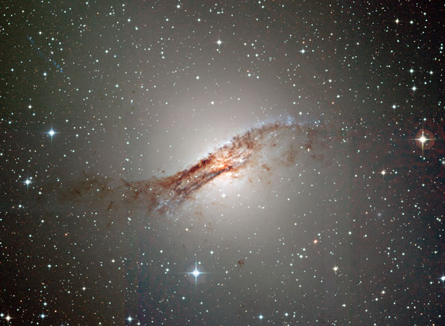
Once I had a clear, or often very blurry, image of an elliptical galaxy, the first step would be to look for evidence of a dust disk. A dust disk is basically exactly what is sounds like, a disk of dust circling the galaxy due to an extremely heavy object pulling it in, most likely a black hole. The problem with black holes is that we cannot analyze them if we cannot see them, so astronomers settle for analyzing the material around them. A clear example of a dust disk in an elliptical galaxy looks like this:

Source

However, my images were hardly that clear on average. A lot of lab time that summer was spent learning how to search in different wavelengths, adjust contrasts, and adjusting wavelength colors to try to get a glimpse of a dust disk. Most of them ended up looking something like this:

Source                                              Source                            Source

And those are normal dust disks. Many of them are distorted by the gravity of another object:

Source

My favorites were the galaxies with two dust disks:

Source

After spending so long looking at questionable candidates finding a nearly perfect dusk disk like the one below was a thing of beauty:

Source

The end results were amazing, but to get there was a lot of tedium. Most of my time was spent searching through NASA databases, making very long spreadsheets of candidates and their properties, and painstakingly adjusting image parameters. By the end of the project I had looked over more than 1,000 galaxies across 6 luminosity "bins."

So many spreadsheets

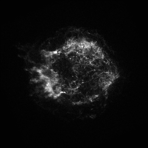
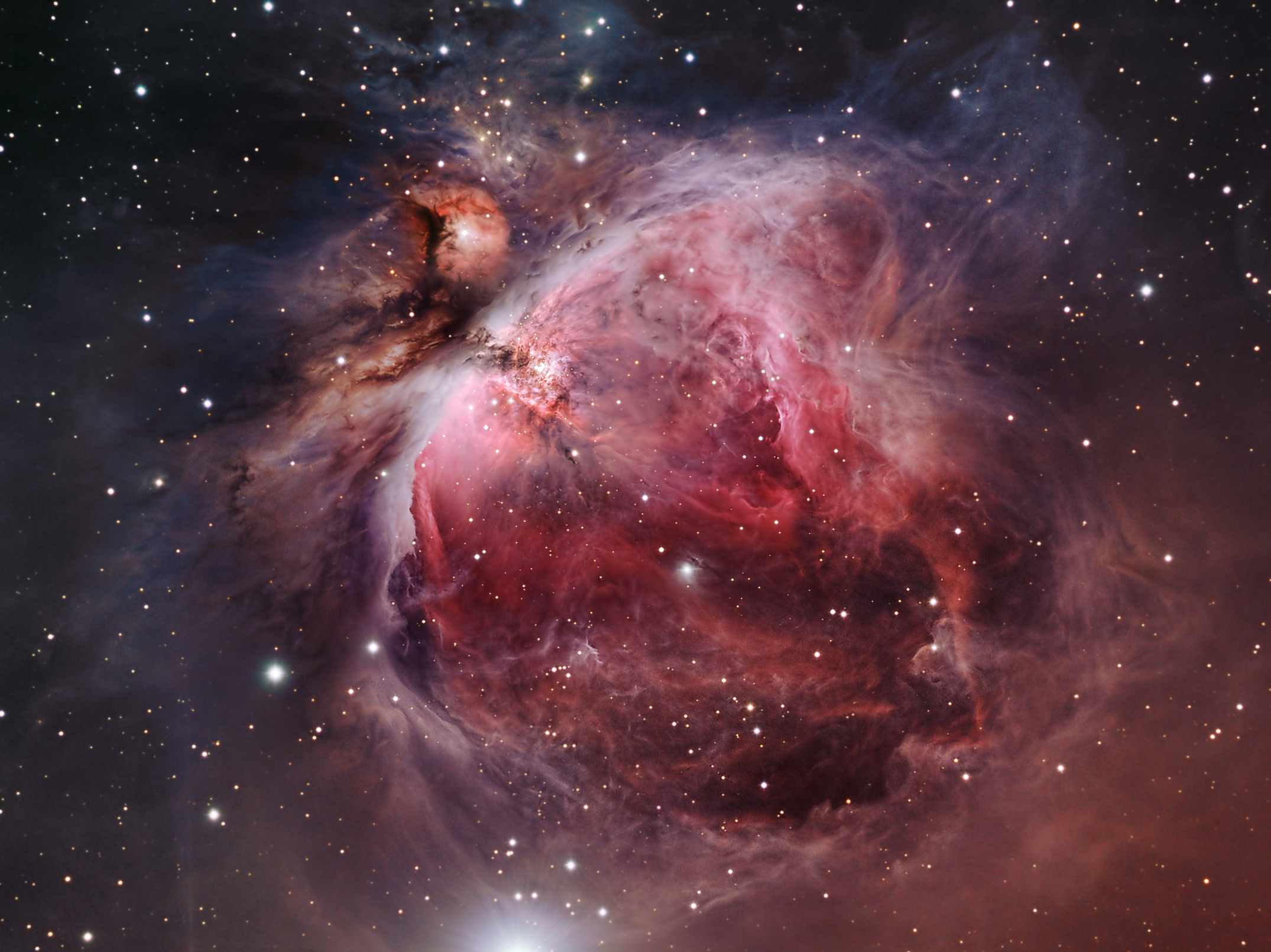
In the end, it is worth it. By analyzing the mass, density, or speed of the dust disk we can begin to collect data on the black hole at the center of the galaxy, something that still mystifies astronomers. Additionally, the project was worth it just because I spent my time looking at gorgeous pictures from the Hubble Space Telescope. Not just of elliptical galaxies but also of exploding supernovae and beauiful spiral galaxies.

 

Source

Source

Additionally, I learned many new things along the way. For example, I constantly saw arcs of light that I could not explain, which is how I first learned about gravitational lensing and some of the crazy effects relativity can have on our observations. I even found evidence for a dust disk in a lensed galaxy.

Source

I finished my project in August of 2014. The professor analyzed the data further in order to write a research proposal. In January of 2015, he wrote me an email to inform me that the project was approved for time on the HUBBLE SPACE TELESCOPE in order to get clearer pictures of some of the better candidates I found. In a few months, the data should be coming in from the telescope and I can't wait to see the pictures.

Source

Overall, those two research projects definitely solidified my interest in astronomy and led me to where I am today: sitting in a Harvard dorm, writing a blog post for Astronomy 17. 

Blog 13: Cecilia Payne-Gaposhkin

Cecilia Payne-Gaposhkin was one of astronomy's most influential researches of the 20th century. Her accomplishments are extremely relevant both to the astronomy we study and to paving the way for female astronomers here at Harvard. 

A portrait Payne-Gaposhkin, which resides on campus at the Harvard Art Museums
Source

Cecilia Payne-Gaposhkin was born in 1900 in Wendover England. She studied natural sciences and botany at Newham College. However, she was so inspired by the work of Arthur Eddington - she had memorized his lecture and could write it verbatim - she switched to the field of astronomy.

In 1919, she came to Radcliffe college with a fellowship designed to encourage women in science at Radcliffe. She went on to receive the first P.h.D. in astronomy from Radcliffe in just two years. Her thesis was described by Otto Struve as "the most brilliant P.h.D. thesis in astronomy." Her work disproved the currently accepted idea that stars are composed of elements similar to Earth. Instead she showed that differences in stellar spectra come from different levels of ionization due to different temperatures, not different chemical compositions. The seven different spectra seen in stars were thought to be different chemical compositions. However, she proposed that due to the hot environments of stars, ions were forming in variable amounts at variable temperatures. This explained the distinct emission spectrum of star types, rather than the idea that there are seven compositionally distinct classes of star. Furthermore, by studying these spectral lines, Payne-Gaposhkin discovered that the abundance of hydrogen and helium is significantly higher in stars than on Earth. The seven different emission patterns perfectly fit with emissions from seven different groups of hydrogen ions, each of which exist in unique temperature ranges. This work paved the way for our modern understanding on element creation via fusion and fission in stars. 

Source

However, her work remained unpublished for years after her dissertation reviewer, astronomer Henry Russell, discouraged her from presenting the findings, as they were too contrary to the accepted cannon. Despite this, Russell published similar findings a few years later and received credit for the discovery.

This did not stop Payne-Gaposhkin. She continued on to study stars of high luminosity, in order to understand the structure of the Milky Way. Additionally, under her direction, 1.25 million observations were made of variable stars, and if that was not enough, another two million observations were made in her study of Magellanic clouds. 

By the end of her life, Payne-Gaposhkin published over 150 papers and recieved an Annie Cannon (another great female astronomer at Harvard) award in 1934. Not only did she recieve the first P.h.D. in astronomy at Radcliffe, she also became the first female full professor in Harvard's Faculty of Arts and Sciences and the first female head of a department at Harvard. Cecilia Payne-Gaposhkin led the way for many astronomers today.

Sources:

http://www.sheisanastronomer.org/index.php/history/cecilia-payne-gaposchkin

http://www.epigenesys.eu/en/science-and-you/women-in-science/808-cecilia-payne-gaposchkin

http://astrogeo.oxfordjournals.org/content/43/1/1.27.full

https://www.youtube.com/watch?v=I_qF-jTY2zY

Reframing Microlensing: Blog 11, Worksheet 4.1, Problem 3

When speaking about microlensing, it is often easier to refer to angular quantities in units of θE. Let’s define u = β/θE and y = θ/θE.

Show that the lens equation can be written as: \[ u = y - y^{-1} \]
A)  Since we know \[ \Theta_E = \left( \frac{4GM_L \pi_{rel} }{ c^2 } \right)^{ \frac{1}{2}} \] and \[ \beta =  \Theta_E - \frac{4GM_L \pi_{rel}}{\Theta c^2} \] we can find \[u =  \frac{ \beta}{\Theta_E} = \frac{\Theta_E - \frac{4GM_L \pi_{rel}}{\Theta c^2} }{\left( \frac{4GM_L \pi_{rel}}{ c^2} \right)^{ \frac{1}{2}} } \] And \[ y = \frac{ \Theta}{\Theta_E} = \frac{\Theta}{ \left(  \frac{4GM_L \pi_{rel} }{ c^2} \right)^{ \frac{1}{2}} } \] Rearranging that gives: \[ u = \frac{ \Theta}{\Theta_E} - \frac{\frac{ \Theta_E^2}{\Theta}}{ \Theta_E} = \frac{ \Theta}{\Theta_E} - \frac{ \Theta_E}{\Theta}= y - y^{-1} \]  \[ u = y - y^{-1} \]

Solve for the roots of y(u) in terms of u. These equations prescribe the angular position of the images as a function of the (mis)alignment between the source and lens. For the situation given in Question 2(f) and a lens-source angular separation of 100 µas (micro-arcseconds), indicate the positions of the images in a drawing.
B)  \[ u = y - y^{-1} \] Multiplying everything by y gives:  \[ yu = y^2 - 1 \] \[ y^2 - uy -1 = 0\] Plugging this into a quadratic equation gives: \[ y = \frac{ u \pm \sqrt{ u^2 + 4} }{2} \] The fact that we have two possible answers is consitent with the two images often seen in gravitational lensing.

Source

In the case of 2(f), we already have \(\beta\) and \( \Theta_E\) so we can rearrange the equation to get:  \[ \frac{ \Theta}{\Theta_E}  = \frac{ \frac{ \beta}{\Theta_E} \pm \sqrt{ \left( \frac{ \beta}{\Theta_E} \right)^2 + 4} }{2} \]  \[ \frac{ \Theta}{1 \times 10^{-6}}  = \frac{ \frac{ 1 \times 10^{-4}}{1 \times 10^{-6}} \pm \sqrt{ \left( \frac{1 \times 10^{-4}}{1 \times 10^{-6}} \right)^2 + 4} }{2} \] \[ \Theta_E = 10^{-4} , -10^{-10} \: arcseconds \] This would look something like this, though this is extremely exaggerated:

The Geometry of Microlensing: Blog 10, Worksheet 4.1, Problem 2

In this part of the worksheet we’re going to do a bunch of geometry to figure out how massive objects can act as Galactic lenses and make background stars brighter through the influence of their gravitational field. The most important scale in lensing is the size of the so-called Einstein ring.

In this part of the worksheet we’re going to do a bunch of geometry to figure out how massive objects can act as Galactic lenses and make background stars brighter through the influence of their gravitational field. The most important scale in lensing is the size of the so-called Einstein ring.

Convince yourself that \( \beta = \Theta -  \alpha' \) , where α' , the source-image angular separation, is distinct from α, the deflection angle of the source, in the figure above. This trivial expression is known as the lens equation.
A) The lens equation makes sense with how each angle is defined in the diagram. I am sufficiently convinced. \[ \beta = \Theta -  \alpha' \]

Next, show that \[ \alpha' = \left( \frac{D_S - D_L }{D_S} \right) \alpha \] and plug it in.
B) Zooming in on specific triangles, we can see that (with a little fudging of distances):

\[ x = sin( \alpha) (D_s - D_L ) =  \alpha (D_s - D_L ) \]

\[ x = sin( \alpha') (D_s ) =  \alpha' (D_s ) \] \[ \alpha' (D_s ) =  \alpha (D_s - D_L )\]

 Plugging in the expression gives: \[ \beta = \Theta -  \left( \frac{D_S - D_L }{D_S} \right) \alpha  \]

Now substitute in the correct expression for α from Question 1(d) to express β in terms of G, ML, b, DL, DS, θ, and c. Remember that you result from 1(d) is a factor of two smaller than the correct expression due to our Newtonian approximations.
C) Using \[ alpha = \frac{4GM_L}{b c^2}\] from question 1, we get: \[ \beta = \Theta -  \frac{2GM_L}{b c^2} \left( \frac{D_S - D_L }{D_S} \right) \] But that if off by a factor of two, due to general relativity, so the equation is really \[ \beta = \Theta -  \frac{4GM_L}{b c^2} \left( \frac{D_S - D_L }{D_S} \right) \]

Replace b with an expression involving θ and DL. Rearrange algebraically to show that \[ \beta = \Theta -  \frac{4GM_L}{\Theta c^2} \left( \frac{D_S - D_L }{D_S D_L} \right) \]
D)

By the small angle approximation we can see that \[sin( \Theta ) = \frac{ b}{D_L} \] \[ b = \Theta D_L \] Plugging this in gives: \[ \beta = \Theta -  \frac{4GM_L}{\Theta c^2} \left( \frac{D_S - D_L }{D_S D_L} \right) \]

When the lens and source lie along the exact same sight line, β “ 0. For this case, solve for the special value of θE, known as the Einstein ring radius, in terms of the lens mass, ML, and the relative parallax, πrel = D^-1 L - D^-1.
E)  \[ \pi_{rel} = D_L^{-1} - D_S^{-1} \] Rearranging \( \pi_{rel} \) gives us a more useful expression.  \[ \pi_{rel} = \frac{D_S  }{D_S D_L} - \frac{D_L }{D_S D_L}= \frac{D_S - D_L }{D_S D_L} \] Plugging in our new information and solving gives:  \[ \beta = \Theta -  \frac{4GM_L}{\Theta c^2} \left( \frac{D_S - D_L }{D_S D_L} \right) \] \[ 0 = \Theta_E -  \frac{4GM_L}{\Theta_E  c^2} \left( \pi_{rel} \right) \] \[ \Theta_E =  \frac{4GM_L}{\Theta_E  c^2} \left( \pi_{rel} \right) \]  \[ \Theta_E = \left( \frac{4GM_L \pi_{rel} }{ c^2 } \right)^{ \frac{1}{2}} \]

For a typical lens of mass 0.3Md (an M-dwarf) at a distance DL = 4 kpc and a typical source at DS = 8 kpc, what is the size of θE in arcseconds?
F)  This is just a matter of plugging in the given information. Converting the givens to cgs gives:

• \(M = 0.3M_{\odot} = 0.6 \times 10^{33} = 6 \times 10^{32} \)
• \( D_L  = 4 \: kpc = 1.2 \times 10^{22} \: cm \)
• \( D_S = 8 \: kpc = 2.5 \times 10^{22} \: cm \)

\[ \Theta_E = \left( \frac{4GM_L  }{ c^2 }  \left( \frac{D_S - D_L }{D_S D_L} \right)  \right)^{ \frac{1}{2}} \] \[ \Theta_E = \left( \frac{4(6.67 \times 10^{-8} )(  6 \times 10^{32}) }{ (3 \times 10^{10})^2 }  \left( \frac{2.5 \times 10^{22} - 1.2 \times 10^{22} }{2.5 \times 10^{22} (1.2 \times 10^{22})} \right)  \right)^{ \frac{1}{2}} \]  \[ \Theta_E = \left( 1.78 \times 10^{5}  \left( 4.33 \times 10^{-23} \right)  \right)^{ \frac{1}{2}} \] \[ \Theta_E = 2.8 \times 10^{-9} radians\] \[ \Theta_E = 1.6 \times 10^{-7} \: degrees = 0.6 \: milli-arcseconds \]

In astronomy, it is often very useful to cast equations in terms of isolated variables measured in units of their typical order-of-magnitude values, with any power law dependencies explicitly labelled for each variable. There should be only one numerical constant out front bearing the proper units for the quantity of interest. This means calculating out all the remaining constants. In equations written in this way, not only can you directly read off the typical numerical value for your quantity of interest, but you can also see exactly how your quantity varies and by how much with changes in each variable.  Recast the equation you derived in 2(f) for θE in terms of the typical lens mass and relative parallax. Your answer should appear in the form: \[ \Theta_E = mas \left( \frac{M_{lens}}{M_{lens \: (typical)}} \right) \left( \frac{\pi_{lens}}{\pi_{lens \: (typical)}} \right) \]

G) \[ \Theta_E = mas \left( \frac{M_{lens}}{M_{lens \: (typical)}} \right) \left( \frac{\pi_{lens}}{\pi_{lens \: (typical)}} \right) \] \[ \Theta_E = 0.6 \: milli-arcseconds  \left( \frac{M_{lens}}{M_{lens \: (typical)}} \right)^{\frac{1}{2}} \left( \frac{\pi_{lens}}{\pi_{lens \: (typical)}} \right)^{\frac{1}{2}} \]  \[ \Theta_E = 0.6 \: milli-arcseconds  \left( \frac{M_{lens}}{6 \times 10^{32} g }   \right)^{\frac{1}{2}} \left( \frac{\pi_{lens}}{4.33 \times 10^{-23} \: mas } \right)^{\frac{1}{2}} \]

That is a lot of information. In the next question, we will convert some of this information into a more accessible format. 

Free form: Blog 8, FERMI (or Frequently Estimated Ridiculous Measuring Inquiries)

This week we learned a lot about dark matter and the mysteries of the universe. These mysteries often have complicated, difficult to remember names. In order to make everyone's lives easier, astronomers often assign acronyms to the objects they discover. This week we have seen some very interesting ones: MAssive Compact Halo Objects (MACHOs) and Weakly Interacting Massive Particles (WIMPs) have invoked some terrific mental pictures of body-building contests. Additionally, we use OGLE (Optical Gravitational Lensing Experiment) to look for MACHOs. The acronyms get more and more far fetched the further you delve into astronomy. A quick google search on my part easily resulted in multiple articles discussing the ridiculous nature of some astronomy acronyms. There is even a blog dedicated to this topic named Dumb Or Overly Forced Astronomy Acronyms Site (DOOFAAS). BeforeI get to the point of this blog post, I would like to share some of my favorite acronyms that I came across in my research:

ARMPIT	ASKAP Rotation Measure and Polarisation InvestigaTion
BICEP	Background Imaging of Cosmic Extragalactic Polarization
BOOMERanG	Balloon Observations Of Millimetric Extragalactic Radiation and Geophysics
COYOTES	Coordinated Observations of Young ObjecTs from Earthbound Sites
FaNTOmM	Fabry-perot of New Technology for the Observatoire du mont Megantic
GADZOOKS!	Gadolinium Antineutrino Detector Zealously Outperforming Old Kamiokande, Super!
MAMBO	MAx-planck-Millimeter-BOlometer
PINOCCHIO	PINpointing Orbit-Crossing Collapsed HIerarchial Objects
POOPSY	Phase One Observing Proposal SYstem
SiEGMuND	Simulation of Events with Geant for Muon and Neutrino Detectors
TANGOinPARIS	Testing Astroparticle with the New Gev/tev Observations Positrons And electRons : Identifying the Sources
WOMBAT	Wavelength-Oriented Microwave Background Analysis Team

That's hardly all of them. There is still MAGIC (MajorAtmospheric Gamma-ray Imaging Cherenkov Telescopes), GANDALF (Gas and Absorption LineFitting), MERLIN (Multi-Element Radio Linked Interferometer Network), ARISTOTELES: Applications and Research Involving Space TechnologiesObserving the Earth's field from Low Earth orbiting Satellite, CANGAROO: Collaboration between Australian and Nippon for a GammaRay Observatory in the Outback. 

Some, I can't believe were approved. For example WISEASS (Weizmann Institute of Science Experimental Astrophysics Spectroscopy System). Here is a link to prove it's real. And SHIT (Super Huge Interferometric Telescope). Here is the link for that one.

Ok, I have had enough fun. Now to the point of the blog post. I would like to propose a Fermi problem: How many acronyms can astronomers possibly make?

Ok, so astronomers have already exceeded my expectations. This blog already has about 400 entries. By estimating from the first thirty or so, the average acronym is 5 letters long. With 26 letters, we can approximate the possible number of letter combinations: \[ 26 \times 26 \times 26 \times 26 \times 26 = 26^5 = 1.2 \times 10^7 \] For a fermi problem this really means our answer is \(10^7\).


We can assume that not all of these combinations make actual words. For example, AAAAA doesn't mean anything to us. I am going to guess that about 10% of combinations make words, in any language that uses our alphabet. But most astronomy happens in English, so I am going to guess that about 10% of those combinations, could be words in English. Therefore, 1% of the words we calculated could make acronyms in English. \[ \frac{10^7}{100} = \boxed{10^5 \: acronyms } \] This is most likely a overestimate, but I am going to keep it because I didn't count the acronyms with numbers (e.g. 5MUSES) or in other languages (e.g. ALMA). 

So how does my answer compare? According to the internet, there are \(2 \times 10^5 \) words in the English dictionary, which means that astronomers can make acronyms of about half the words in the dictionary. They better get cracking on that. Good thing there are nearly infinite things to discover in outer space.

Sources:
https://www.cfa.harvard.edu/~gpetitpas/Links/Astroacro.html
http://space.io9.com/an-alphabet-soup-of-absurd-astronomy-acronyms-1613063426
http://www.space.com/28244-strange-astronomy-acronyms.html

Mass of the Milky Way: Blog 7, Worksheet 3.1, Problem 6

Now consider a spherically symmetric galaxy with a density profile: \[ ρ(r) = \frac{C}{ 4πr^2(r + a )^2 } \] where a and C are constants. 

(a) What is M(< r ) for this galaxy? You can leave your answer in terms of C and a. 
\[ ρ(r) = \frac{C}{ 4πr^2(r + a )^2 } \] We know from the previous problem that \[\frac{dM}{dr} = 4 \pi r^2 \rho (r) \] Combining this information gives: \[\frac{dM}{dr} = 4 \pi r^2 \left( \frac{C}{ 4πr^2(r + a )^2 } \right) \]  And now we can solve for M \[\frac{dM}{dr} = \frac{C}{(r + a )^2} \]  \[dM = \frac{C}{(r + a )^2}dr \]  \[\int dM = \int_{0}^{r} \frac{C}{(r + a )^2}dr \] \[M(r) = - \frac{C}{(r + a ) } |_{0}^{r} = \frac{ - C}{r + a } + \frac{C}{r + a}\] \[ M = \frac{Cr}{a^2 + ar} \]
(b) The total mass of the system is the the limit of M(< r ) as r --> \(\infty\); calculate this total mass. 
\[lim_{x\to\infty} \frac{Cr}{a^2 + ar} = \frac{\infty}{\infty} \] That is not very helpful for the sake of this problem. In order to solve this, we can think back to high school calculus and invoke L'Hopital's rule, which tells us that in the case that the limit of the top and bottom equal infinity, the limit derivative of the top and bottom of the fraction will equal the limit of the fraction: \[lim_{x\to\infty} \frac{C}{a} \] \[M_{tot} = \frac{C}{a}\]

(c) If we write the total mass as Mtot, rewrite M(< r ) and ρ(r) to eliminate C in favor of Mtot. 

This problem is just a matter of combining two equations we already know: \[1) \: M_{tot} = \frac{C}{a}\] can also be written as \[C = a \times M_{tot}\] and \[2) \:  ρ(r) = \frac{C}{ 4πr^2(r + a )^2 } \] Substituting for C gives: \[ ρ(r) = \frac{a  M_{tot}}{ 4πr^2(r + a )^2 } \]

(d) What is the rotation curve v(r) for this galaxy? You should find that the circular velocity goes to a constant as r --> 0, i.e., at radii r << a, this galaxy appears to have a flat rotation curve. If we write this constant velocity as Vo, write M(< r ) and ρ(r) in terms of Vo, a, and r. What is Mtot in terms of Vo and a? 

We can use the formulas we have for density to solve for velocity: \[ \rho (r)  = \frac{ V_c^2}{4 \pi r^2 G} =  \frac{a  M_{tot}}{ 4πr^2(r + a )^2 } \] \[ V_c^2 = \frac{Ga  M_{tot}}{(r+a)^2}\]  \[ V_c = \left( \frac{Ga  M_{tot}}{(r+a)^2} \right)^{\frac{1}{2}} \] Now we can find the limit of \(V_c\) to get \(V_0\) when r<<a. \[ lim_{r\ to 0}V_c = \left( \frac{Ga  M_{tot}}{a^2} \right)^{\frac{1}{2}} \] This means: \[V_0^2 = \frac{GM_{tot}}{a^2} \] Now we want to rewrite M(< r) and ρ(r) in terms of Vo, a, and r. For M(< r), we only really need to get rid of C  \[ M = \frac{Cr}{a^2 + ar} \] We can use the equation derived above for Vo to find \( M_{tot} \) \[\boxed{M_{tot} = \frac{V_0^2 a}{G}} \] setting this equal to our equation for \( M_{tot} \) in part b gives: \[ \frac{C}{a} = \frac{V_0^2 a}{G} \] \[C = \frac{V_0^2 a^2}{G} \] \[M(r) = \frac{Cr}{a^2 + ar} = \frac{V_0^2 a^2 r}{G (a^2 + ar)} \] \[ \boxed{M(r) =\frac{V_0^2 ar}{Ga + Gr}} \] \[ \boxed{ ρ(r) = \frac{V_0^2 a^2}{ G4πr^2(r + a )^2 } } \]

(e) If we consider this as a model of the Milky Way, what is a in kpc if Mtot = \( 10^{12} M_{\odot} \) and Vo = 240 km/s?

For this last problem, we can just plug and chug. In cgs, \(V_0 = 2.4 \times 10^7 \) cm/s and \(M_{\odot} = 2 \times 10^{33} g \).

Solving the \(M_{tot} \) formula for a gives: \[ a = \frac{GM_{tot}}{V_0^2} = \frac{(6.67 \times 10^{-8})(10^{12} \times 10^{33} ) }{(2.4 \times 10^7)^2 }= 1.2 \times 10^{23} \: cm \approx 40 \: kpc  \]

Mass Density of the Galaxy: Blog 6, Worksheet 3.1, Problem 5

We know something suspicious is happening with the mass of the galaxy in our approximations. A good next step is to check related variables and see if they are suspicious too. A good example is density:

M(r < r) is related to the mass density ρ(r) by the integral: \[ M(< r) = \int_{0}^{r}  4π'^{2} ρ(r') dr'\](Recall that the \(4πr^{2} \) comes from the surface area of each spherical shell, and the dr' is the thickness of each thin shell; talk to a TF if this is not clear.) The fundamental theorem of calculus then implies that 4πr^2ρ(r) = dM(< r)/dr. For the case in question 4, what is ρ(r)? Is the density finite as r --> 0 in the case of a flat rotation curve?

The Milky Way's rotation curve 

Source

This calculation is simply a matter of using what we already know. We have from question 4: \[M(r) = \frac{ V_c^2 r }{G} \] Taking the derivative gives us: \[\frac{dM}{dr} = \frac{ V_c^2}{G} \] which we can set equal to \[\frac{dM}{dr} = 4 \pi r^2 \rho (r) \] And solve for density. \[4 \pi r^2 \rho (r)  = \frac{ V_c^2}{G} \] \[ \rho (r)  = \frac{ V_c^2}{4 \pi r^2 G} \]

This calculated density would be infinite in the case of a flat rotation curve.

Rotation Curves: Blog 6, Worksheet 3.1, Problem 4

This week we went further into our exploration of the Milky Way, but something didn't quite add up. The mass of observable matter in the galaxy, does not actually match the mass of the galaxy. This is the basic idea that lead to the astronomical mystery of dark matter. For this weeks three blog posts, I will type up questions 4-6 on worksheet 3.1, because they flow well together and build evidence that the mass of the galaxy is not quite what we think. The first step of this is measuring the rotation curve of the galaxy:

We actually observe a flat rotation curve in our own Milky Way. (You will show this with a radio telescope in your second lab!) This means v(r) is nearly constant for a large range of distances. 

(a) Lets call this constant rotational velocity Vc. If the mass distribution of the Milky Way is spherically symmetric, what must be the M(< r) as a function of r in this case, in terms of Vc, r, and G? 


In question number three we found a formula for the Keplerian rotation curve, v(r) for a mass m if the central mass is concentrated in a single point at the center (with mass Menc). The formula we found for that problem ended up being \[ v^2 = \frac{G M_{enc} }{r} \] Rearranging this formula for this specific question leads us to: \[M(< r) = \frac{ V_c^2 r }{G} \]

(b) How does this compare with the picture of the galaxy you drew last week with most of the mass appearing to be in bulge? 

This approximation assumes the mass of the galaxy is constant as you go out from the center. We know that is not true because there is a quite heavy bulge in the middle of the milky way.

Source

(c) If the Milky Way rotation curve is observed to be flat (Vc < 240 km/s) out to 100 kpc, what is the total mass enclosed within 100 kpc? How does this compare with the mass in stars? Recall the total mass of stars in the Milky Way, a number you have been given in your first assignment and should commit to memory.

In our first assignment we learned that the mass of the Milky Way is \(10^{10} M_{\odot} \). Lets see how our calculations compare: \[ M_{MW} = 10^{10} M_{\odot} = 10^{10} \times 2 \times 10^{33} = 2 \times 10^{43} \: grams \] \[M(< 100 \: kpc) =  \frac{ V_c^2 r }{G} = \frac{ (240)^2 (2 \times 10^{43}) }{6.67 \times 10^{-8}} = 8.6 \times 10^{54} \: grams \]
That is a huge discrepancy between the two masses. Something suspicious is afoot...

Supernovas and Sandra Bullock: Blog 5, Worksheet 2.1, Problem 4

A supernova goes off and you can barely detect it with your eyes. Astronomers tell you that supernovae have a luminosity of 1042 erg/s; what is the distance of the supernova? Assume the supernova emits most of its energy at the peak of the eye’s sensitivity and that it explodes isotropically. 

The light exploding isotropically and hitting our eye would look something like this:

So we can begin to set up this problem.

What we know:

• We know the speed of light is \(3 \cdot 10^{10} \frac{cm}{sec}\)
• E = hν
• \(P = \frac{\delta E}{\delta t}\)
• Visible light falls into a range between 390 - 700 nm, which an average could be 6.0 x \(10^{-7}\) cm.
• The radius of an eye is about 1 cm.
• The "refresh rate" of a movie is 50 Hz.
• The luminosity of the supernova is \( 10^{42} \) erg/s.

Solve:

Based on the fact that the light is emitted isotropically (shown partially in the diagram above), we can set up a ratio between the power emitted by the supernova over the area the light reaches to the power received by your eye to the area of your eye.\[\frac{P_{s}}{a_{light}} = \frac{P_{eye}}{a_{eye}}\]plugging in area formulas gives:\[\frac{P_{s}}{4 \pi d^2} = \frac{P_{eye}}{\pi r_{eye}^2}\] Solving for distance gives :\[d^2 = \frac{P_{s}\cdot r_{eye}^2}{4 \cdot  P_{eye} }\]

Now we all we need to find is the power reaching our eye, starting with finding the energy.  \[E = hv \: or \: E = h\frac{c}{\lambda} = 6.6 x 10^{-27} \cdot \frac{3 x 10^{10}}{6.0 x 10^{-7}} \approx 3.3x10^{-10} ergs\]

Now we need to find time. Something new I learned last semester, when we solved a similar problem, was  refresh rate, or the rate at which movies emit light so that the brain does not notice any flickering in the movie. If the refresh rate of a movie is 50 Hz (\( \frac{1}{s}\)) and 10 photons must hit the eye every \( \frac{1}{50}\)s, so we need 500 photons a second. So the power would be  \[ P = \frac{500 photons}{sec} \cdot 3.3x10^{-10} ergs \approx 1.65x10^{-7} \frac{erg}{s}\] Plugging this into the original equation (and keeping in mind power is just luminosity) we get: \[d^2 = \frac{10^{42} \cdot 1^2}{ 4 \cdot 1.65x10^{-7} } \] \[ d = 1.2 \times 10^{24} cm \: or \: 3.6 \times 10^5 pc\] This seems like a reasonable distance for a supernova.

Blackbodies and Flux: Blog 4, Worksheet 2.1, Problem 3

You observe a star you measure its flux to be \(F_{\star} \). If the luminosity of the star is \(L_{\star} \) 
(a) Give an expression for how far away the star is. 

Flux is energy per time per area, so we know that at a distance, d, flux is: \[F_{\star}= \frac{L_{\star}}{4 \pi d^2 } \] Solving for d gives: \[d^2 = \frac{ L_{\star} }{4 \pi  F_{\star} } \]  \[d = \left( \frac{ L_{\star} }{4 \pi  F_{\star} } \right)^{ \frac{1}{2}} \]

(b) What is its parallax? 

In the first worksheet we found the relationship: \[ \theta = \frac{ 1 \: AU }{d} \] Substituting for d gives: \[ \theta =  \left( \frac{ 4 \pi  F_{\star} }{L_{\star} } \right)^{ \frac{1}{2}} \] with parsecs that would be \[ \theta =  \frac{1}{2 \times 10^5} \left( \frac{ 4 \pi  F_{\star} }{L_{\star} } \right)^{ \frac{1}{2}} \]

(c) If the peak wavelength of its emission is at λo, what is the star’s temperature? 

In question 1 we found: \[ \lambda_0 = \frac{hc}{4kT} \] solving for T gives: \[ T = \frac{hc}{4k \lambda_0} \]

(d) What is the star’s radius, \(R_{\star} \)?

For this, we can use the relationship: \[ L_{\star} = 4 \pi R^2 T^4 \] Solving for R gives \[ R = \left( \frac{L_{\star}}{4 \pi \sigma T^4 } \right)^{\frac{1}{2}} \] Substituting for T gives:   \[ R = \left( \frac{L_{\star}k^4 \lambda_0^4 }{64 \pi \sigma h^4 c^4 } \right)^{\frac{1}{2}}\]

Drawing Our Galaxy: Worksheet 1.2, Problem 1

Create an illustration of the Milky Way galaxy as viewed from outside the galaxy, viewed from the side and from above. You can draw by hand, or use a digital drawing tool such as Google Draw, Gimp or Illustrator. Post your illustration as a blog post, along with descriptive text of the figure. Your audience is a high school senior interested in astronomy, so don’t let them down with an obfuscated or incorrect description! Be sure to include the components in the list below. You may use any resource you find on the internet, but be sure that you have two sources for each bit of information you find so as to not post embarrassingly erroneous information. Wikipedia provides pretty solid information, but you should use library books, lecture notes, online books and/or Youtube videos as supporting information.
(a) Location of the Sun
(b) Thin/thick disks, bulge, halo
(c) Globular clusters
(d) The Small Magellanic Cloud (SMC) and the Large Magellanic Cloud (LMC)
(e) Sgr A* (Black hole)
(f) Location of Orion star forming region, and the nearest and furthest (known) open clusters to the Sun
(g) Scale length and scale height (in order to draw galaxy to scale)

Above we see a depiction - or at least an attempt at one - of our home. In astronomy 16, we focused on more immediate surroundings: stars and planets. In astronomy 17 we will be dealing with much bigger scales, and what better way to begin than with our home galaxy. The milky way galaxy is about 30 kilo-parsec in diameter, or at least most of the stars are within that diameter. There is also the "scale length" of the milky way to describe the width that contains the majority of the stars. The scale length is 3.5 kilo-parsecs and the scale height is 0.3 kilo-parsecs. Around the milky way there is a spherical halo, aptly named the halo, extending at least 40 kilo-parsecs and containing old stars, a little dust, and globular clusters (dense groups of stars).

In the middle of the galaxy lies the black hole Sgr A* with a radius of 22.5 million kilometers. Around the black hole is the bulge, made mainly of old stars, gas, and dust. Moving out from the bulge is the disk of the milky way. There is a thick disk that is about 1 kilo-parsec high and a thin disk about 300 pc high. This is where the spiral arms are located, with younger stars in the thin disk and older stars in the thick disk, on average.

We live in the Orion arm of the milky way, 8 kilo-parsec out from the center of the galaxy. Within one kilo-parsec of our sun (and therefore too nearby to fit in the diagram) lie the orion star forming region, Hyades, and Berkeley 29. The orion star forming region contains the orion nebula, a nursery for baby stars and one of the most photographed objects in space:

Source

Hyades is the nearest known open cluster - or a group of a few thousand stars that formed from the same molecular cloud - to the sun. It is about 47 parsecs away. The furthest known open cluster in the milky way is Berkeley 29 and is 15,000 parsecs away.

The Small Magellanic Cloud and the Large Magellanic Cloud are two galaxies in our milky way's neighborhood, or local group, that can be seen from the southern hemisphere. They are classified in some places as dwarf galaxies and in others as Magellanic galaxies: dwarf galaxies with one arm. The LMC is 50 kilo-parsecs away and 4.3 kilo-parsecs in diameter. The SMC is 61 kilo-parsecs away and 2.1 kilo-parsecs in diameter. 

Hope you enjoyed this tour of our neighborhood! Enjoy this complimentary map for all of you galactic travels.

Milkomeda: Blog 2, Worksheet 1.1, Problems 2-4

The Andromeda Galaxy and the Milky Way Galaxy are slowly but surely colliding into the charmingly named Milkomeda Galaxy. In the first worksheet of the semester, we did a few calculations to learn more about Milkomeda.

Source

Problem 2: . How long will it take for Andromeda to collide with the Milky Way? The time-scale here is the free-fall time, tff. One way of finding this is to assume that Andromeda is on a highly elliptical orbit (e -> 1) around the Milky Way. With this assumption, we can use Kepler’s Third Law \[P^2 = \frac{4 \pi^2 a^3}{G (M_{MW} + M_{And} )} \] where P is the period of the orbit and a is the semi-major axis. How does \(t_{ff}\) relate to the period? Estimate it to an order of magnitude.

We can approximate an e --> 1 ellipse as almost a straight line.

Therefore, we can approximate the free fall time of the second galaxy as half of the period of rotation, as it must fall approximately the length of the orbit. \[t_{ff} = \frac{P}{2}\] Plugging this into the given equation for period allows us to approximate free fall time: \[(2t_{ff})^2 \approx \frac{4 \pi^2 a^3}{G (M_{MW} + M_{And} )} \] \[ t_{ff} \approx \left( \frac{ \pi^2 a^3}{G (M_{MW} + M_{And} )} \right)^{\frac{1}{2}} \] Now it is just a matter of plugging in constants, all of which we were given on the worksheet: \[a \approx 400 kpc \approx 1.24 \times 10^{24} cm \] \[M_{\odot} \approx 10^{33} g \] \[M_{MW} + M_{And} \approx 2 \times 10^{12} M_{\odot} \approx 2 \times 10^{45} g  \] \[G \approx 6.68 \times 10^{-8} \] \[ t_{ff} \approx \left( \frac{ \pi^2 (1.24 \times 10^{24})^3}{6.68 \times 10^{-8} (2 \times 10^{45})} \right)^{\frac{1}{2}} \] \[t_{ff} = 3.75 \times 10^{17} \: seconds \] \[1.2 \times 10^{10} years\]

Problem 3: Let’s estimate the average number density of stars throughout the Milky Way, n. First, we need to clarify the distribution of stars. Stars are concentrated in the center of the galaxy, and their density decreases exponentially: \[ n(r) \propto e^{\frac{-r}{R_s}} \] is also known as the “scale radius” of the galaxy. The Milky Way has a scale radius of 3.5 kpc. With this in mind, estimate n in two ways: 
(a) Consider that within a 2 pc radius of the Sun there are five stars: the Sun, α Centauri A and B, Proxima Centauri, and Barnard’s Star. 

We can approach this problem by approximating the galaxy with the 2pc radius around the Sun. The density of stars in the described reason would be: \[ n = density = \frac{ stars}{volume} = \frac{5}{ \frac{4}{3} \pi 2^3 } \approx 0.149 \frac{stars}{pc^3} \] According to google, we are 8 kpc from the center of the universe, which is about 2 scale radii from the center of the galaxy. For the sake of not doing an integral, we can approximate. With every scale radii, the function drop by \( \frac{1}{e} \), so at 2 radii it has dropped by about \( \frac{1}{e^2} \). To account for this, we can just multiply our density by e^2: \[0.149 \frac{stars}{pc^3} \times e^2 \approx 1.10 \frac{stars}{pc^3}  \]

(b) The Galaxy’s “scale height” is 330 pc. Use the galaxy’s scale lengths as the lengths of the volume within the Galaxy containing most of the stars. Assume a typical stellar mass of 0.5\(M_{\odot}\).

To find number density we need, by definition, the number of stars in the galaxy and the volume of the galaxy. To get the number of stars we need to divide the mass of the galaxy by the average mass of a star: \[ \frac{M_{galaxy}}{M_{star}} = \frac{10^{10} M_{\odot} }{ .5 M_{\odot} } = 2 \times 10^{10} stars \] To get volume, we can approximate the galaxy as a cylinder, assuming most stars are within one scale radius of the center.

 \[ V = (3500)^2 \times \pi \times 300 = 1.27 \times 10^{10} pc^3 \] Now that we have both pieces, we can solve for n: \[ n = \frac{N}{V} = \frac{2 \times 10^{10} stars}{1.27 \times 10^{10} pc^3} = 1.57 \frac{ stars}{ pc^3} \]

Problem 4: Determine the collision rate of the stars using the number density of the stars (n), the cross-section for a star \(σ_{\star}\), and the average velocity of Milkomeda’s stars as they collide v. How many stars will collide every year? Is the Sun safe, or likely to collide with another star?

We know collision rate is proportional to velocity, area, and number density. Using dimensional analysis, we can solve for the actual equation \[collision \: rate \: \propto \:v \: σ \: n  \] \[ \frac{stars}{time} = \frac{cm}{s} \times cm^2 \times \frac{stars}{cm^3} \] All the units cancel so the equation would be \[collision \: rate  = v \: σ \: n \] We know all pieces of this equation, but need to do a few calculations. To find velocity we can use the distance and time from problem 2: \[ v = \frac{d}{t_{ff}} =  \frac{ 2.5 \times 10^{24} }{2 \times 10^{18} } = 1.25 \times 10^6 cm/s \] We can convert our n to cgs: \[ 1.6 \times \frac{1}{(3 \times 10^{18})^3} = 6 \times 10^{-56} \frac{stars}{cm^3} \]  If we approximate our sun as an average star in the galaxy, we have the last piece of this puzzle, cross sectional area. Now we can solve: \[ collision \: rate  = v \: σ \: n  = (1.25 \times 10^6 ) \pi (7 \times 10^{10} )^2 (6 \times 10^{-56}) \approx 1 \times 10^{-27} \frac{stars}{s} \] Multiplying that answer by how many seconds there are in a year ( \( 3.2 \times 10^7  \) s ) tells us that there are \(3.4 \times 10^{-20} \) collisions per year. It is pretty unlikely that the sun will hit anything anytime soon. So we can all breathe a sigh of relief.

Intro Post - Round 2

Hello Universe!

Or rather, welcome back. My name is Danielle Frostig and I took Astronomy 16 last spring. Here is a link to my previous introduction. I won't bore you by repeating everything I wrote there. Instead, I will share what is new.

General life updates: I am no longer a wide-eyed freshman living in Weld Hall, but rather a seasoned sophomore living in Quincy House. I am still planning on majoring in Astrophysics, and at some point this semester, I will have to officially declare my concentration. I had a fun summer with lots of travel going to Israel, home to California, and to China. This leads me to...

Astronomy life updates: In China I got to teach astronomy to about fifty Chinese high school students. It was a lot of fun and an interesting challenge to teach astronomy in Beijing, where it is too polluted to see stars. Additionally, I happened to be in Los Angeles the day all the Pluto data was coming in from the New Horizons mission. While at the Griffith Observatory, I had the chance to see the data coming in and hear from lead scientists about their new discoveries. My favorite thing I learned about that day was the crazy, chaotic orbit of one of Pluto's moon's, Nix.

Source

Here's to the new semester!

Danielle