Geometry of the Universe: Blog 31: Worksheet 10.1, Question 2

Ratio of circumference to radius.
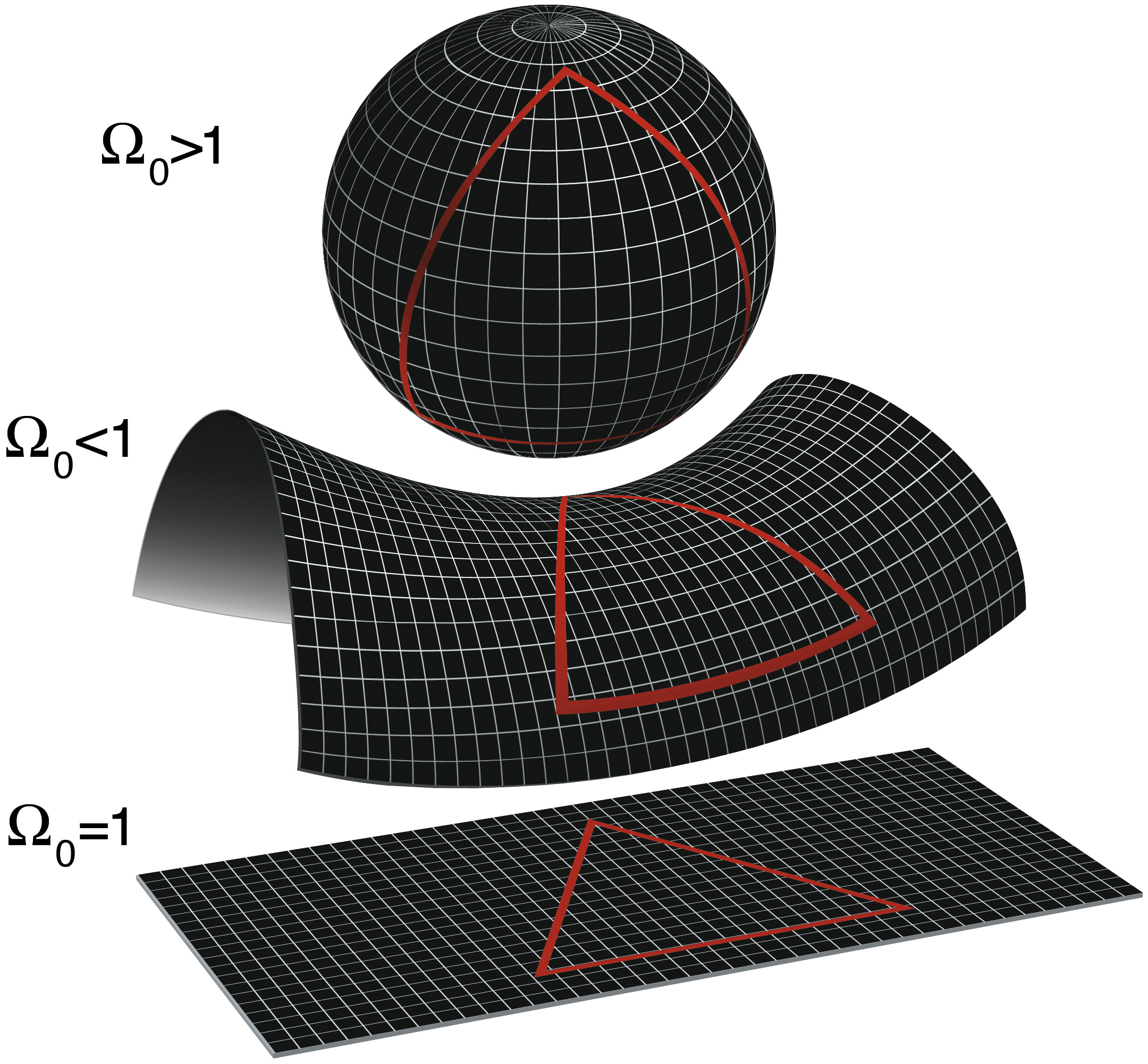
Let’s continue to study the difference between closed, flat and open geometries by computing the ratio between the circumference and radius of a circle.

(a) To compute the radius and circumference of a circle, we look at the spatial part of the metric and concentrate on the two-dimensional part by setting dφ = 0 because a circle encloses a two-dimensional surface. For the flat case, this part is just \[ ds_{2d}^2 = dr^2 + r^2 dθ^2\] The circumference is found by fixing the radial coordinate (r = R and dr = 0) and both sides of the equation (note that θ is integrated from 0 to 2π). The radius is found by fixing the angular coordinate (θ, dθ = 0) and integrating both sides (note that dr is integrated from 0 to R). Compute the circumference and radius to reproduce the famous Euclidean ratio 2π.

With these new definitions of R and dr, our relationship is:  \[ ds_{2d}^2 = 0 + R^2 dθ^2\] or \[ ds_{2d} = R dθ\] Taking the integral of each side gives us an expression for circumference:  \[ \int_0^C ds = \int_0^{2 \pi} R dθ\] \[ C = 2 \pi R \] This looks pretty familiar, now we can move on to less familiar geometries. \[ \frac{C}{R} = \frac{2 \pi R}{R} = 2 \pi \]

(b) For a closed geometry, we calculated the analogous two-dimensional part of the metric in Problem (1). This can be written as: \[ds_{2d}^2 = dξ^2 + sin(ξ)^2 dθ^2\] Repeat the same calculation above and derive the ratio for the closed geometry. Compare your results to the flat (Euclidean) case; which ratio is larger? (You can try some arbitrary values of ξ to get some examples.)

Radius:
With these new definitions of R and dr, the metric goes from: \[ds_{2d}^2 = dξ^2 + sin(ξ)^2 (dθ^2 + sin(θ)^2 d \phi^2) \] to \[ds_{2d}^2 = dξ^2 \]  or \[ ds_{2d} = dξ\] Taking the indefinite integral of each side gives us an expression for radius: \[ \int ds_{2d} = \int dξ\] \[ s =  ξ = R \]
Circumference:
Once again, our relationship simplifies nicely. \[ds_{2d}^2 = dξ^2 + sin(ξ)^2 dθ^2\]  \[ds_{2d}^2 = sin(ξ)^2 dθ^2 \] \[ds_{2d} = sin(ξ) dθ \] Taking the integral with the outlined bounds to find circumference:   \[ \int_0^C ds = \int_0^{2 \pi} sin(ξ)  dθ\] \[ C = 2 \pi sin(ξ)  \] This expression is less familiar to us, but does resemble \( C = 2 \pi R\) with our definition of R in this case.
Ratio: \[ \frac{C}{R} = \frac{2 \pi sin(ξ)}{ξ}  \] Because this circumference is dependent on a sine term, the circumference will never be greater than \( 2 \pi \) or less than \( -2 \pi \) so this ratio will always be equal to or less than the ratio found in Euclidian Space in part a.

(c) Repeat the same analyses for the open geometry, and comparing to the flat case.

Radius:
In an open geometry, the procedure for radius is the same. \[ds_{2d}^2 = dξ^2 + sin(ξ)^2 (dθ^2 + sin(θ)^2 d \phi^2) \] \[ ds_{2d} = dξ\]  \[ \int ds_{2d} = \int dξ\] \[ s =  ξ = R \] Circumference: In the metric for open geometry is R = sinh(x) so the metric simplifies to  \[ds_{2d}^2 = sinh(ξ)^2 dθ^2 \]  \[ \int_0^C ds = \int_0^{2 \pi} sinh(ξ)  dθ\] \[ C = 2 \pi sinh(ξ)  \] Ratio:  \[ \frac{C}{R} = \frac{2 \pi sinh(ξ)}{ξ}  \] This ratio will always be larger or equal to the ratio in the flat, and closed universe.

(d) You may have noticed that, except for the flat case, this ratio is not a constant value. However, in both the open and closed case, there is a limit where the ratio approaches the flat case. Which limit is that?

The two ratios we found are :  \[ \frac{C}{R} = \frac{2 \pi sin(ξ)}{ξ}  \] \[ \frac{C}{R} = \frac{2 \pi sinh(ξ)}{ξ}  \] As we approach 0, we can use the small angle approximation for both of these functions, (e.g. sin(ξ) is ξ) so as the limit goes to zero, both ratios go to zero, approaching the flat case (this is easy to visualize in the graph above). In class, Ashley compared this geometry to us being small human beings on a large Earth. On the whole, we know the Earth is a three-dimensional sphere, but at small scales, as the limit approaches zero, the Earth looks flat.

Representations of the three types on universes - Source

Blog 30: Galactic Rotation

Next week we will begin our second lab of the semester. We will use the millimeter-wave telescope, a radio telescope, in order to observe giant molecular clouds in the Milky Way. This is a lot of new information at once, so we are going to answer some questions before we actually head to lab.

Why? - We are observing GMCs in order to find their redshifts. From redshift, we can find the velocity of a GMC along our line of sight. With that velocity, we can find the circular velocity of a GMC rotating in the Milky Way using \[ V_{cir} = V_r(max) + V_{\odot} sin(l) \] where Vr is the radial velocity of the GMC moving away from us and the second term is the velocity of the sun in the direction of the cloud.

In previous blog posts  we explored why the rotation curve of the galaxy is important in astronomy. The basic idea is that we observe objects to be rotating too quickly, too far out in the galaxy just based on visible matter. This is our main indicator that there is another type of dark matter in the universe. Additionally, we can learn more about the Milky Way's visible matter from this experiment. For example, we can estimate the number of stars in the galaxy. 

How? - The telescope will detect radiation at the wavelength near 2.6 mm, or a frequency of 115.271 GHz. This wavelength corresponds with a strong emission line of Carbon Monoxide. We will obtain this spectrum from the telescope's spectrometer, one of many of the telescope's parts among an antenna for collecting and focusing the signal, a liquid helium cooler, and a computer for recording and interpreting data.

What is going to be the typical integration time per point? - What integration time would be needed to detect the peak of 12CO with SNR = 10 if I use a filter bank with 256 channels that are 0.5 MHz wide. TA for CO is about 2-3 K and Tsys = 500K?

In worksheet 9.2 we found \[ \tau = \frac{ SNR^2 T_{sys}^2 }{T_A^2 \Delta \nu } \] \[ \tau = \frac{ (10)^2 (500)^2 }{(2.5)^2 (0.5 \times 10^6) } \approx 8 \: seconds \]

Over what range of longitude do you plan to observe? - We are planning on observing from \(10^{\circ} \: \text{ to } 70^{\circ} \). 

How many positions do you plan to observe? - We plan on observing 4 GMCs, so we will most likely observe 4 positions.

At what LST are you going to start observing? At what EST? - I have been assigned to Monday's lab from 11:00 - 3:00 EST. Let's say that means we start observing at 11:30 EST. The LST on that date and time at our longitude (71.11 degrees west) would be 15:55.

Additionally, we can solve question number two on the worksheet to learn more about the experiment.  

Resolution of a single dish radio telescope: The spatial resolution of a telescope is θ = 1.2 λ/D , where D is the diameter of the dish, and λ is the observing wavelength. In radio astronomy, θ is also known as the half-power beam width (or full-width half-max of the beam). 

(a) Find an equation for the beam width, in arcminutes, of a single-dish radio in terms of frequency ν in GHz, and diameter D in meters. Use a calculator to determine this to 1 decimal place. Write an equation of the form \[ \theta = degrees \left( \frac{ \nu}{GHz} \right)^{-1} \left( \frac{D}{m} \right)^{-1} \] We can solve this by redefining theta: \[ \theta = \frac{c}{\nu D} = \frac{1.2 (3 \times 10^8) }{(1 \times 10^9)(1)} = 0.36 \: rad \left( \frac{180^{\circ}}{ \pi rad } \right) = 20.6^{\circ} \] \[ \theta = 20.6^{\circ} \left( \frac{ \nu}{GHz} \right)^{-1} \left( \frac{D}{m} \right)^{-1} \] 

(b) What is the beamwidth, in arcminutes, for the CfA 1.2 m telescope at the 12CO frequency?

Using the formula we just found, we know \[ \theta = 20.6^{\circ} \left( \frac{ \nu}{GHz} \right)^{-1} \left( \frac{D}{m} \right)^{-1} \] \[ \theta = 20.6^{\circ} \left( \frac{ 115.271 \: GHz}{GHz} \right)^{-1} \left( \frac{1.2 \: m}{m} \right)^{-1} = 0.149^{\circ} = 8.95 \: arcminutes \] 

(c) What linear dimension in pc does this correspond to at the Galactic center (8.5 kpc)?

We can call on our trusty parallax formula for this problem: \[ d = \frac{1}{ \theta} \] Where 8.95 arcminutes is 537 arcseconds, so \[ d = \frac{1}{ 537} = 1.9 \times 10^{-3} \: pc \] Now we should be all set to start lab.

Correction: The parallax is not a terribly useful number in this case. Rather the question is asking for resolvable size, which we could find with simple trigonometry. \[sin( \theta) = \frac{l}{8.5 \: kpc} \] With the small angle approximation, this is \[ l \approx 0.149 \cdot \frac{\pi}{180} \cdot 8,500 \approx 22 \: pc\]

More Friedmann Equations: Blog 29, Worksheet 9.1, Problem 2

GR modification to Newtonian Friedmann Equation:

In Question 1, you have derived the Friedmann Equation in a matter-only universe in the Newtonian approach. That is, you now have an equation that describes the rate of change of the size of the universe, should the universe be made of matter (this includes stars, gas, and dark matter) and nothing else. Of course, the universe is not quite so simple. In this question we’ll introduce the full Friedmann equation which describes a universe that contains matter, radiation and/or dark energy. We will also see some correction terms to the Newtonian derivation.

A) The full Friedmann equations follow from Einstein’s GR, which we will not go through in this course. Analogous to the equations that we derived in Question 1, the full Friedmann equations express the expansion/contraction rate of the scale factor of the universe in terms of the properties of the content in the universe, such as the density, pressure and cosmological constant. We will directly quote the equations below and study some important consequences. Use the first Friedmann equation: \[ \left( \frac{\dot{a}}{a} \right)^2 = \frac{8 \pi}{3} G \rho + \frac{ \kappa c^2 }{a^2} + \frac{ \Lambda }{3} \] and the second Friedmann equation: \[ \frac{\ddot{a}}{a}  = - \frac{4 \pi G}{3c^2} ( \rho c^2 + 3P) + \frac{ \Lambda }{3} \] To find the third equation in a flat universe \[ \dot{ \rho} c^2 = -3 \frac{\dot{a}}{a}( \rho c^2 + P) \]

With the universe being flat and multiplying the first equation by acceleration squared gives us: \[ \ddot{a}^2 = \frac{8 \pi}{3} G \rho a^2+ \frac{ \Lambda }{3} a^2 \] Taking the time derivative gives us \[ 2 \dot{a} \ddot{a} = \frac{8 \pi}{3} G \dot{\rho} a^2 + \frac{16 \pi}{3} G \rho \dot{a} a   + \frac{2  \Lambda }{3} \dot{a} a \] Rearranging this allows us to set it equal to the second equation: \[  \frac{ \ddot{a} }{a} = \frac{4 \pi a}{3  \dot{a} } G \dot{\rho}  + \frac{ 8 \pi}{3} G \rho + \frac{ \Lambda }{3} =  - \frac{4 \pi G}{3c^2} ( \rho c^2 + 3P) + \frac{ \Lambda }{3} \] Which simplifies with a few cancellations to: \[ \dot{ \rho} c^2 = -3 \frac{\dot{a}}{a}( \rho c^2 + P) \]

B) Cold matter dominated universe. If the matter is cold, its pressure P = 0, and the cosmological constant Λ = 0. Use the third Friedmann equation to derive the evolution of the density of the matter ρ as a function of the scale factor of the universe a. You can leave this equation in terms of ρ, ρ0, a and a0, where ρ0 and a0 are current values of the mass density and scale factor. The result you got has the following simple interpretation. The cold matter behaves like “cosmological dust” and it is pressureless (not to be confused with warm/hot dust in the interstellar medium!). As the universe expands, the mass of each dust particle is fixed, but the number density of the dust is diluted - inversely proportional to the volume. Using the relation between ρ and a that you just derived and the first Friedmann equation, derive the differential equation for the scale factor a for the matter dominated universe. Solve 2 Astronomy 17 - Galactic and Extragalactic Astronomy Fall 2015 this differentiation equation to show that \(a(t) \propto t^{\frac{3}{2}}\) . This is the characteristic expansion history of the universe if it is dominated by matter.

Without pressure, the third equation can be written as \[ \frac{\dot{\rho}}{\rho} = -3 \frac{\dot{a}}{a}\] Taking the derivative of both sides with respect to time starting at \( \rho_0 \: \text{and} \: a_0 \) produces:  \[ \frac{\rho}{\rho_0} = \left(\frac{a}{a_0} \right)^{-3}\] Plugging this relationship into the first equation gives: \[ \left( \frac{\dot{a}}{a} \right)^2 = \frac{8 \pi}{3} G \left( \frac{a_0^3 \rho_0}{a^3} \right) \] Taking the derivative of each side gives \[ a^{\frac{1}{2}} = c \: dt \] Where c is a constant (because we just want a relationship between a and t). Taking the integral of each side gives \[ \frac{2}{3} a^{\frac{3}{2} } = c t \] So \[ a(t) \propto t^{\frac{3}{2}} \]

C) Radiation dominated universe. Let us repeat the above exercise for a universe filled with radiation only. For radiation, \(P = \frac{1}{ 3} ρc^2 \)and Λ = 0. Again, use the third Friedmann equation to see how the density of the radiation changes as a function of scale factor. The result also has a simple interpretation. Imagine the radiation being a collection of photons. Similar to the matter case, the number density of the photon is diluted, inversely proportional to the volume. Now the difference is that, in contrast to the dust particle, each photon can be thought of as wave. As you learned last week, the wavelength of the photon is also stretched as the universe expands, proportional to the scale factor of the universe. According to quantum mechanics, the energy of each photon is inversely proportional to its wavelength: E = hν. Unlike the dust case where each particle has a fixed energy. So in an expanding universe, the energy of each photon is decreasing inversely proportional to the scale factor. Check that this understanding is consistent with the result you got. Again using the relation between ρ and a and the first Friedmann equation to show that \(a(t) \propto t^{\frac{1}{2}}\) for the radiation only universe.

With the new pressure, the third equation can be written as \[ \frac{\dot{\rho}}{\rho} = -4 \frac{\dot{a}}{a}\] Taking the derivative of both sides with respect to time starting at \( \rho_0 \: \text{and} \: a_0 \) produces:  \[ \frac{\rho}{\rho_0} = \left(\frac{a}{a_0} \right)^{-4}\] Plugging this relationship into the first equation gives: \[ \left( \frac{\dot{a}}{a} \right)^2 = \frac{8 \pi}{3} G \left( \frac{a_0^4 \rho_0}{a^4} \right) \] Taking the derivative of each side gives \[ a = c \: dt \] Where c is a constant (because we just want a relationship between a and t). Taking the integral of each side gives \[ \frac{1}{2} a^{2 } = c t \] So \[ a(t) \propto t^{\frac{1}{2}} \]

D) Cosmological constant/dark energy dominated universe. Imagine a universe dominated by the cosmological-constant-like term. Namely in the Friedmann equation, we can set ρ = 0 and P = 0 and only keep Λ nonzero. As a digression, notice that we said “cosmological-constant-like” term. This is because the effect of the cosmological constant may be mimicked by a special content of the universe which has a negative pressure \(P = - ρc^2 \). Check that the effect of this content on the right-hand-side of third Friedmann equation is exactly like that of the cosmological constant. To be general we call this content the Dark Energy. How does the energy density of the dark energy change in time? Show that the scale factor of the cosmological-constant-dominated universe expands exponentially in time. What is the Hubble parameter of this universe?

From the first equation we have: \[ \left( \frac{\dot{a}}{a} \right)^2 =  \frac{ \Lambda }{3} \] Taking the derivative gives: \[ \frac{da}{a} = \sqrt{ \frac{ \Lambda }{3} } dt \] Ignoring constants, the integral of this relationship turns into \[ ln(a) \propto t \] \[ a \propto e^t \] And because \[ H=  \frac{\dot{a}}{a} \] The Hubble constant in this universe is  \[ H = \sqrt{ \frac{ \Lambda }{3} } \]

E) Suppose the energy density of a universe at its very early time is dominated by half matter and half radiation. (This is in fact the case for our universe 13.7 billion years ago and only 60 thousand years after the Big Bang.) As the universe keeps expanding, which content, radiation or matter, will become the dominant component? Why?

Radiation will dominate because it falls off at a slower rate ( \(a(t) \propto t^{\frac{1}{2}}\) ) than matter ( \(a(t) \propto t^{\frac{2}{3}}\) ).

F) Suppose the energy density of a universe is dominated by similar amount of matter and dark energy. (This is the case for our universe today. Today our universe is roughly 68% in dark energy and 32% in matter, including 28% dark matter and 5% usual matter, which is why it is acceleratedly expanding today.) As the universe keeps expanding, which content, matter or the dark energy, will become the dominant component? Why? What is the fate of our universe?

Dark energy will be dominant as the universe expands and matter is scattered. Energy, and therefore normal matter, cannot be created or destroyed, by the law of conservation of energy. We have also shown that dark energy will increase at a faster rate ( \(a \propto e^t\) ) than radiation ( \(a(t) \propto t^{\frac{2}{3}}\) ). Eventually, our universe will be a very sparse, vast expanse of dark energy with few pockets of matter spread throughout.

Cosmology: Blog 28, Worksheet 9.1, Problem 1

A Matter-only Model of the Universe in Newtonian Approach 

In this exercise, we will derive the first and second Friedmann equations of a homogeneous, isotropic and matter-only universe. We use the Newtonian approach. Consider a universe filled with matter which has a mass density ρ(t). Note that as the universe expands or contracts, the density of the matter changes with time, which is why it is a function of time t. Now consider a mass shell of radius R within this universe. The total mass of the matter enclosed by this shell is M. In the case we consider (homogeneous and isotropic universe), there is no shell crossing, so M is a constant.

(a) What is the acceleration of this shell? Express the acceleration as the time derivative of velocity,  \( \dot{v} \)(pronounced v-dot) to avoid confusion with the scale factor a (which you learned about last week).

Because this acceleration is due to gravity, we know \[ ma  = F_g \] \[ m\dot{v} = - \frac{GMm}{R^2} \] \[ \dot{v} = - \frac{GM}{R^2} \]

(b) To derive an energy equation, it is a common trick to multiply both sides of your acceleration equation by v. You should arrive at the following equation: \[ \frac{1}{2} \dot{R}^2 - \frac{GM}{R} = C \]

Using what we found in a: \[ \frac{dR}{dt} \dot{v} = - \frac{GM}{R^2} \frac{dR}{dt} \] Which simplifies to \[v \: dv = - \frac{GM}{R^2} dR \] The integral of this is \[ \frac{1}{2} v^2 = \frac{GM}{R} + C \] Where C is a constant. Substituting \( v = \dot{R} \) we have: \[ \frac{1}{2} \dot{R}^2 - \frac{GM}{R} = C \]

(c) Express the total mass M using the mass density, and plug it into the above equation. Rearrange your equation to give an expression for \( \left( \frac{ \dot{R}}{R} \right)^2 \), where \(  \dot{R} = \frac{dR}{dt}  \). \[ M = \rho V = \frac{4}{3} \pi R^3 \rho \] Plugging this into our expression from part B gives us:  \[ \frac{1}{2} \dot{R}^2 - \frac{G \left( \frac{4}{3} \pi R^3 \rho \right)}{R} = C \] Rearranging this makes it: \[ \left( \frac{\dot{R}}{R} \right)^2 = \frac{2C}{R^2} + \frac{8 \pi G}{3} \rho (t) \]

(d) R is the physical radius of the sphere. It is often convenient to express R as R = a(t)r, where r is the comoving radius of the sphere. The comoving coordinate for a fixed shell remains constant in time. The time dependence of R is captured by the scale factor a(t). The comoving radius equals to the physical radius at the epoch when a(t) = 1. Rewrite your equation in terms of the comoving radius, R, and the scale factor, a(t). \[  \frac{\dot{R}}{R} =  \frac{\dot{a}(t) r}{a(t) r} =  \frac{\dot{a}}{a} \] So our expression is  \[ \left( \frac{\dot{a}}{a} \right)^2 = \frac{2C}{R^2} + \frac{8 \pi G}{3} \rho (t) \]

(e) Rewrite the above expression so that \( \left( \frac{\dot{a}}{a} \right)^2 \) appears alone on the left side of the equation. \[ \checkmark \]

(f) Derive the first Friedmann Equation: From the previous worksheet, we know that \( H(t) =  \frac{\dot{a}}{a} \). Plugging this relation into your above result and identifying the constant \( \frac{2C}{r} = \kappa c^2 \) where k is the “curvature” parameter, you will get the first Friedmann equation. The Friedmann equation tells us about how the shell of expands or contracts; in other words, it tells us about the Hubble expansion (or contracration) rate of the universe. \[ \left( \frac{\dot{a}}{a} \right)^2 = \frac{8 \pi}{3} G \rho - \frac{ \kappa c^2 }{a^2} \]

(g) Derive the second Friedmann Equation: Now express the acceleration of the shell in terms of the density of the universe, and replace R with R = a(t)r. You should see that a: \( \frac{\ddot{a}}{a}  = - \frac{4 \pi G}{3c^2} \rho \), which is known as the second Friedmann equation. The more complete second Friedmann equation actually has another term involving the pressure following from Einstein’s general relativity (GR), which is not captured in the Newtonian derivation. If the matter is cold, its pressure is zero. Otherwise, if it is warm or hot, we will need to consider the effect of the pressure.
\[ \dot{v} = - \frac{GM}{R^2} = -\frac{4}{3} \pi G \rho (t) a(t) r \] We know \( \dot{v} = \ddot{R} \) so \(  \dot{v} = \ddot{a}r \) and \[\ddot{a}r = -\frac{4}{3} \pi G \rho (t) a(t) r \]  \[ \frac{\ddot{a}}{a}  = - \frac{4 \pi G}{3c^2} ( \rho c^2 + 3P) + \frac{ \Lambda }{3} \]

The Age and Size of the Universe: Blog 27: Worksheet 8.1, Problem 3

It is not strictly correct to associate this ubiquitous distance-dependent redshift we observe with the velocity of the galaxies (at very large separations, Hubble’s Law gives ‘velocities’ that exceeds the speed of light and becomes poorly defined). What we have measured is the cosmological redshift, which is actually due to the overall expansion of the universe itself. This phenomenon is dubbed the Hubble Flow, and it is due to space itself being stretched in an expanding universe. Since everything seems to be getting away from us, you might be tempted to imagine we are located at the centre of this expansion. But, as you explored in the opening thought experiment, in actuality, everything is rushing away from everything else, everywhere in the universe, in the same way. So, an alien astronomer observing the motion of galaxies in its locality would arrive at the same conclusions we do. In cosmology, the scale factor, a(t), is a dimensionless parameter that characterizes the size of the universe and the amount of space in between grid points in the universe at time t. In the current epoch, t = \(t_0\) and \( a(t)_0 = 1\) a(t) is a function of time. It changes over time, and it was smaller in the past (since the universe is expanding). This means that two galaxies in the Hubble Flow separated by distance \(d_0 = d(t_0) \) in the present were \(d(t) = a(t)d_0 \)apart at time t. The Hubble Constant is also a function of time, and is defined so as to characterize the fractional rate of change of the scale factor: \[H(t) = \frac{1}{a(t)} \frac{ da}{ dt}|_t \] and the Hubble Law is locally valid for any t: \[v = H(t)d\] where v is the relative recessional velocity between two points and d the distance that separates them.

Part A: Assume the rate of expansion, a = da/dt, has been constant for all time. How long ago was the Big Bang (i.e. when a(t=0) = 0)? How does this compare with the age of the oldest globular clusters (= 12 Gyr)? What you will calculate is known as the Hubble Time.

Since we know \[v = H(t)d\] \[H(t) = \frac{v}{d} = \frac{1}{t} \] So \[ t_0 = \frac{1}{H(t)} = \frac{1}{68.816 \frac{km/s}{Mpc}} = 0.01453 \frac{Mpc \cdot s}{km} \] This is not a very useful number for us, so we can convert it to years: \[ 0.01453 \frac{Mpc \cdot s}{km} \cdot \frac{ 3.086 \times 10^{19} \: km}{Mpc} \cdot \frac{ 1 year }{3.15 \times 10^7}  = 1.385 \times 10^{10} \: years \] This is pretty close! The actual age of the universe is 13.82 billion years. This means the oldest globular clusters formed less than 2 billion years after the big bang.

Part B:  What is the size of the observable universe? What you will calculate is known as the Hubble Length.

Once again, we know \[ v = H(t)d\] So, if the universe is expanding at the speed of light and the speed of light in km/s is \( 3 \times 10^{5} \). \[ d = \frac{c}{H(t)} \] \[ d = \frac{3 \times 10^{5}}{68.816} = 4,356 Mpc \approx 4 \times 10^{3} Mpc \] The actual size of the universe is about \( 3 \times 10^{3} \) Mpc, so we aren't too far off.

Our old friends, Lyman-alphas: Blog 24 & 25, Worksheet 7.2, Problem 4 & 5

This week, we learned about active galactic nuclei and all of their fun applications. One of those applications in particular is especially dear to me, because the summer before tenth grade, I did a research project (and wrote a blog post about it) in a lab where I calculated the distance to ancient galaxies using redshift from Lyman-alpha emitting active galactic nuclei. And wouldn't you know, that's what we're doing in class this week:

Problem 4

One feature you surely noticed in a spectrum was the strong, broad emission lines. Here is a closer look at the strongest emission line in the spectrum:

This feature arises from hydrogen gas in the accretion disk. The photons radiated during the accretion process are constantly ionizing nearby hydrogen atoms. So there are many free protons and electrons in the disk. When one of these protons comes close enough to an electron, they recombine into a new hydrogen atom, and the electron will lose energy until it reaches the lowest allowed energy state, labeled n = 1 in the model of the hydrogen atom shown below (and called the ground state):

On its way to the ground state, the electron passes through other allowed energy states (called excited states). Technically speaking, atoms have an infinite number of allowed energy states, but electrons spend most of their time occupying those of lowest energies, and so only the n = 2 and n = 3 excited states are shown above for simplicity. Because the difference in energy between, e.g., the n = 2 and n = 1 states are always the same, the electron always loses the same amount of energy when it passes between them. Thus, the photon it emits during this process will always have the same wavelength. For the hydrogen atom, the energy difference between the n = 2 and n = 1 energy levels is 10.19 eV, corresponding to a photon wavelength of λ = 1215.67 Angstroms. This is the most commonly-observed atomic transition in all of astronomy, as hydrogen is by far the most abundant element in the Universe. It is referred to as the Lyman α transition (or Lyα for short). It turns out that that strongest emission feature you observed in the quasar spectrum above arises from Lyα emission from material orbiting around the central black hole.

Part A: Recall the Doppler equation: \[ \frac{ \lambda_{observed} - \lambda_{emitted}}{\lambda_{emitted}} = z \approx \frac{v}{c} \]Using the data provided, calculate the redshift of this quasar. \[ z =  \frac{ 1410 - 1215.67}{1215.67} \approx \frac{1}{6}  \] So that \[ v \approx \frac{c}{6}\]

Part B: Again using the data provided, along with the Virial Theorem, estimate the mass of the black hole in this quasar. It will help to know that the typical accretion disk around a \(10^8 M_{\odot} \) black hole extends to a radius of r = \(10^{15} \) m. 

Ideally, our emission lines would be infinitely thin and tall, but they have width. This happens because there is some dispersion due to the rotation of the galaxy. This means some of the galaxy will be redshifted and some will be blueshifted. 

So we can use this to find rotational velocity.

\[ z = \frac{ \lambda_{observed} - \lambda_{emitted}}{\lambda_{emitted}} = \frac{1415 - 1406}{1406} \approx 0.00640 \]

\[ z = \frac{1415 - 1406}{1406} = 0.0064 \] \[ v \approx 0.0064 c \]

Now we can use the virial theorem: \[ K = - \frac{1}{2} U \] \[ Mv^2 = \frac{G M^2}{R}\] \[M_{BH} = \frac{ v^2 R}{G} = \frac{( 0.0064 \cdot 3 \times 10^{10})^2 (10^{17})}{6.67 \times 10^{-8}} = 5.5 \times 10^{40} \: g \approx 3 \times 10^7 M_{\odot} \] 

Problem 5

You may also have noticed some weak “dips” (or absorption features) in the spectrum:

Part A: Suggest some plausible origins for these features. By way of inspiration, you may want to consider what might occur if the bright light from this quasar’s accretion disk encounters some gaseous material on its way to Earth. That gaseous material will definitely contain hydrogen, and those hydrogen atoms will probably have electrons occupying the lowest allowed energy state.

As the question implies, we are probably looking at instances where light is being absorbed or emitted by hydrogen gas on its way to us. These dips themselves, occurring before the peak, imply that this gas is between the galaxy and us, therefore they are not as redshifted as the distant galaxy. 

Part B: A spectrum of a different quasar is shown below. Assuming the strongest emission line you see here is due to Lyα, what is the approximate redshift of this object?

\[ \frac{ \lambda_{observed} - \lambda_{emitted}}{\lambda_{emitted}} = z \approx \frac{v}{c} \]

\[ z = \frac{5650 - 1215.67}{1215.67} = 3.347 \approx 3\]

Part C: What is the most noticeable difference between this spectrum and the spectrum of 3C 273? What conclusion might we draw regarding the incidence of gas in the early Universe as compared to the nearby Universe?

In this galaxy, there are many more variation, especially a larger number of deeper "dips." Based on the large redshift of the galaxy, we know it is quite old and far away. This means the light had to have traveled through a lot more gas to get here, and some of that gas had hydrogen atoms occupying the lowest energy state. Additionally, this could tell us that there was a lot more gas in the early universe. This fits in well with our current ideas of the early universe. 

Deriving Hubble's Law: Blog 26: Worksheet 8.1: Problem 2

In 1929, astronomer Edwin Hubble discovered that almost all distant galaxies exhibit a positive redshift. Furthermore, it appeared that the farther the galaxy, the larger its redshift. Here we will rediscover Hubble’s Law using modern spectroscopic data and supernovae Ia as our distance indicator to these galaxies. The data we will use come from the Sloan Digital Sky Survey (SDSS), a project that aims to comprehensively map the universe. You can access the relevant data products for this exercise at http://goo.gl/fmIvqc

Part A: Below is a list of supernovae observed between 2004 and 2007 and their positions in RA and Dec. You can find the images and spectra of their host galaxies by entering their coordinates in the respective fields. Explore the functions available, including magnifying the image, reading off the photometric measurements (magnitudes in wavebands u, g, r, i, z) of your selected object, and using the ‘Explore’ button to access more quantitative measurements for these objects. In particular, familiarize yourself with the ‘interactive spectrum’ feature.

For each galaxy, we have a pretty extensive spectrum.

Part B: One of the features for determining distances to Type Ia supernovae is its peak absolute magnitude. You explored the peak bolometric luminosities of SN Ia’s in Worksheet 7.1. The peak V-band magnitude for SN Ia’s is about -19.3. Use the apparent peak magnitudes given in the table above to calculate the distance of these supernovae in unit of Mpc.

To find distance, we can use our trusty distance formula :\[d = 10^{ \frac{m - M + 5}{5}} \] for each magnitude. The fourth galaxy did not have a spectrum associated with it, so we did not analyze it.

Part C: We can use the absorption or emission lines of the host galaxy to find their redshifts which, as you found in Question 1), roughly equals the recessional velocity as a fraction of the speed of light. To measure the redshift to each host galaxies, click on ‘Explore’ and then on the link ‘Interactive Spectrum’. Uncheck the boxes Best Fit and Mark Emission Lines. Zoom in on the absorption line labeled Hα, and move your mouse over to the center of the line to read the observed wavelength in Angstroms. The Hα has a rest (i.e. emitted) wavelength of 6563.0 Angstroms. Calculate the redshift, and then derive the radial velocity in kilometers per second, using the relation z = v/c. How close does your redshift measurements compare to the one SDSS reports in the table under the Interactive Spectrum link? Repeat for all the galaxies.

We found redshift and velocity using \[ \frac{ \lambda_{observed} - \lambda_{emitted}}{\lambda_{emitted}} = z \approx \frac{v}{c} \] to find: 

Part D: Make a plot of your findings, with distance on the x-axis and velocity on the y-axis. Report the slope of your line in appropriate units. This is the Hubble Constant, H0.

Result: \(H_0 = 68.816 \frac{km/s}{Mpc} \)

Part E: Write an equation for this line in the form of v = ___ D, where v is an object’s recessional velocity and D is the distance to that object. Express your Hubble Constant in terms of units km/s/Mpc. Congratulations, you have arrived at Hubble’s Law!
\[ v = 68.816 \frac{km/s}{Mpc} D \] Now we have a basic law of the universe (kinda) down!