Worksheet 12.2, Problem 2: Goldilocks Zone

The Problem: The Earth resides in a “Goldilocks Zone” or habitable zone (HZ) around the Sun. At our semimajor axis we receive just enough Sunlight to prevent the planet from freezing over and not too much to boil off our oceans. Not too cold, not too hot. Just right. In this problem we’ll calculate how the temperature of a planet, Tp, depends on the properties of the central star and the orbital properties of the planet.

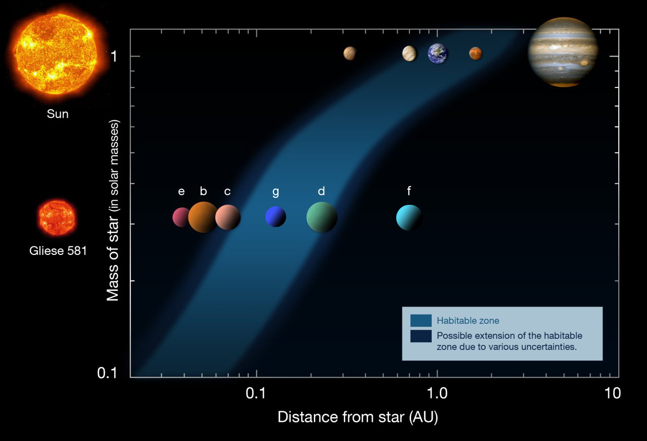
This image gives a good overall preview to the Goldilocks Zone and the factors that we will ultimately calculate that influence it.

Source

Part A: Draw the Sun on the left, and a planet on the right, separated by a distance a.

Part B: Due to energy conservation, the amount of energy received per unit time by the planet is equal to the energy emitted isotropically under the assumption that it is a blackbody.

How much energy per time does the planet receive from the star?

We used dimensional analysis to remind ourselves that the units for luminosity is  \( \frac{erg}{s} \) so: \[L_{\star} = \frac{E_{\star} }{t} \] Based on the question, we then deduced the energy per time the planet receives would be \[\frac{E_p }{t} = \frac{L_{\star} }{4 \pi a^2} \cdot \pi R_p^2 \] Where \(\pi R_p^2\) is the cross-sectional area of the planet that receives light and heat from the star (a circle). So this is  \[\frac{E_p }{t} = \frac{L_{\star} R_p^2 }{4 a^2}\]

How much energy per time does the Earth radiate as a blackbody?

Treating Earth as a blackbody would give: \[\frac{E_p }{t} = 4 \pi \sigma R_p^2 T_p^4 \]We know this from when we worked with blackbodies some weeks ago.

Part C: Set these two quantities equal to each other and solve for TP .
\[\frac{L_{\star} R_p^2 }{4 a^2} = 4 \pi \sigma R_p^2 T_p^4 \] When we isolate T we get \[T_p^4 = \frac{L_{\star}}{16 \sigma a^2} \] Or \[T_p= \left( \frac{L_{\star}}{16 \sigma a^2} \right)^{\frac{1}{4}}\]

Part D: How does the temperature change if the planet were much larger or much smaller?

The temperature would not change. We know this 1) because the radius of the planet is in our equation and 2) logically, any change in size of a planet would be negligible compared to the distance of the planet from the star and should not make a difference.

Part E: Not all of the energy incident on the planet will be absorbed. Some fraction, A, will be reflected back out into space. How does this affect the amount of energy received per unit time, and thus how does this affect Tp?

The temperature lost due to reflected energy would be \[T_p^4 = \frac{L_{\star}A}{16 \sigma a^2} \] So the total temperature would be \[T_p^4 = \frac{L_{\star}}{16 \sigma a^2} - \frac{L_{\star}A}{16 \sigma a^2} \] Or \[\frac{L_{\star}(1-A)}{16 \sigma a^2} \] And T would scale to \[T_p \sim (1-A)^{\frac{1}{4}} \]

I worked with Sean, April, and Barra on this problem.

Worksheet 12.1: Problem 5: Squiggles Abound

The problem: Assuming the core temperature, TC, of a Sun-like star is pretty much constant (nuclear fusion is a threshold process with a steep temperature dependence on the reaction rate), what are the following relationships?

Part A: Mass-radius

We know the equation of state and can simplify from there: \[P_c = \frac{ \rho \kappa T }{\bar{m}} \] Taking out the constants gives us \[ P \sim \rho T \]  \[\rho T \sim \frac{M^2}{R^4} \] We know \[ \rho = \frac{M}{R^3}\] so \[\frac{M^2}{R^4}  \sim \frac{M}{R^3}\] and finally \[M \sim R \]

Part B: Mass-luminosity (L = Mα) for massive stars M > Mo, assuming the opacity (cross-section per unit mass) is independent of temperature κ = const.

From question 3 we know \[L \sim \frac{T_c^4  R}{\kappa \rho} \] When we take out the constants, this gives, \[L \sim \frac{ R}{ \rho} \] Once again using \(\rho = \frac{M}{R^3} \) and \(M \sim R \) from above lets us simplify to \[L \sim \frac{ R}{ \frac{M}{R^3}}\] \[ L \sim M^3 \]

Part C: Mass-luminosity for low-mass stars M < 1 Mo, assuming the opacity (cross-section per unit mass) scales as κ = ρT^3.5 . This is the so-called Kramer’s Law opacity.

Once again we can use \(L \sim \frac{T_c^4  R}{\kappa \rho} \) but this time \(\kappa\) is not constant so \[L \sim \frac{T_c^{7.5} R}{\rho^2} \] And one more time using \(\rho = \frac{M}{R^3} \) and \(M \sim R \) we can simplify to \[ L \sim \frac{R}{\rho^2} \sim \frac{R}{\frac{M^2}{R^6}} \sim \frac{R^7}{M^2}\] \[L \sim M^5\] 

Part D: Luminosity-effective temperature \( T_{eff}^4  \sim L^{\alpha} \) for the two mass regimes above. This locus of points in the T-L plane is the so-called Hertzsprung-Russell (H–R) diagram. Sketch this as log L on the y-axis, and log Teff running backwards on the x-axis. It runs backwards because this diagram used to be luminosity vs. B-V color, and astronomers don’t like to change anything. Include numbers on each axis over a range of two orders of magnitude in stellar mass (0.1 < M < 10 Mo). For your blog post, look up a sample H-R diagram showing real data using Google Images. How does the slope of the observed H-R diagram compare to yours?

For both cases we know \[T_{eff} = \frac{L}{4 \pi R_{\star}^2} \] which scales to \[T_{eff}^4 \sim \frac{L}{R_{\star}^2} \] which is really \[T_{eff}^4  \sim \frac{L}{M_{\star}^2} \] 

For high mass stars, we know \(L \sim M^3\) so \[T_{eff}^4  \sim \frac{L}{L^{\frac{2}{3}}} \] \[T_{eff}^4  \sim L^{\frac{1}{3}} \] 

For low mass stars, we know \(L \sim M^5\) so: \[T_{eff}^4  \sim \frac{L}{L^{\frac{2}{5}}} \] \[T_{eff}^4  \sim L^{\frac{3}{5}} \]

For simplicity, in this class we will use the average \(L \sim M^4 \) and \(L \sim T^8 \). Plotting this against two log scales gives:

Which is roughly in line with an actual HR diagram:

Source

I worked with Sean, Barra, and April on this problem.

Write about anything?

For my free blog post I thought I would write about something cool I stumbled across that is happening here at Harvard, more specifically at the Harvard Art Museum. Before I even get to my point, I have to say that if you haven't been to our art museum, please go. It's right on campus and has works by amazing artists, including Monet, Picasso, Cezanne, Dali, Polluck, Rubens, and Miro, just to name a few.

Look at how close it is.

I actually have a point, I promise. In the art museum, we have many majestic, ancient, white marble statues such as the one of Hypatia below:

Source

However, these statues weren't always monochromatic. At some point, each statue was brightly painted (they even had noses at some point). A group of art historians used paint chips left of sculptures along with UV scans to figure out what colors some ancient art pieces were originally painted, and here are the results:

Source

Although this exhibit is no longer featured at our art museum, research is continuously happening. In the mean time, the recreations are causing quite a stir. Some like seeing the art in its original intention, while others say the bright colors ruin the elegant image of ancient art. What do you prefer?

*Bonus fun fact: some of the ancient roman statues show evidence of having once been painted with bright, colorful hair, suggesting that the ancient romans used colorful dyes in their own hair.

Worksheet 11.2, Problem 1: Flow of Energy

The problem: Stars generate their energy in their cores, where nuclear fusion is taking place. The energy generated is eventually radiated out at the star’s surface. Therefore, there exists a gradient in energy density from the center (high) to the surface (low), but thermodynamic systems tend towards ‘equilibrium.’ In the following sections we will determine how energy flows through the star.

Part A: Inside the star, consider a mass shell of width ∆r, at a radius r. This mass shell has an energy density u + ∆u, and the next mass shell out (at radius r + ∆r) will have an energy density u. Both shells behave as blackbodies.

The net outwards flow of energy, L(r), must equal the total excess energy in the inner shell divided by the amount of time needed to cross the shell’s width ∆r. Use this to derive an expression for L(r) in terms of du/dr , the energy density profile. This is the diffusion equation describing the outward flow of energy.

Once again, an image from the textbook can help us visualize the situation.

Source

If we keep in mind the answer needs to be in terms of du/dr we can solve: \[L(r) = \frac{dE}{dt} = \frac{dE}{du}\frac{du}{dt} = \frac{dE}{dt}\frac{du}{dr}\frac{dr}{dt} \] We can simplify this because you know \[ \frac{dE}{du} = 4 \pi r^2 dr \] and \[ \frac{dr}{dt} = v \] and \[v = \frac{c}{\rho \kappa \Delta r} \] \[L(r) = 4 \pi r^2 \frac{c}{\rho \kappa} \frac{du}{dr} \]

Part B: From the diffusion equation, use the fact that the energy density of a blackbody is u(T(r)) = aT^4 to derive the differential equation: \[\frac{dT(r)}{ dr} \propto - \frac{ L(r) \kappa \rho (r)}{ πr^2acT^3}\] where a is the radiation constant. You just derived the equation for radiative energy transport!

\[u(T(r)) = aT^4\] \[ du(T(r)) = 4aT^3 d(T(r)) \] From part a: \[du = \frac{L(r) \rho \kappa dr}{4 \pi r^2 c } \] So \[\frac{L(r) \rho \kappa dr}{4 \pi r^2 c } =  4aT^3 d(T(r)) \] Which simplifies to our answer!  \[\frac{dT(r)}{ dr} \propto - \frac{ L(r) \kappa \rho (r)}{ πr^2acT^3}\]

Acknowledgements: I worked on this worksheet with Sean, April, and Barra.

Worksheet 11.1: Photons Random Walking Out of a Star

 The problem: Consider a photon that has just been created via a nuclear reaction in the center of the Sun. The photon now starts a long and arduous journey to the Earth to be enjoyed by Ay16 students studying on a nice Spring day.

Source

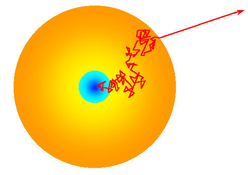
Part A: The photon does not travel freely from the Sun’s center to the surface. Instead it random walks, one collision at a time. Each step of the random walk traverses an average distance l, also known as the mean free path. On average, how many steps does the photon take to travel a distance ∆r? 

We know that on average, the displacement for random walk journeys would be zero, which is not very useful to us. Instead, we can look at the displacement squared:\[ < \vec{ D }^2> = \sum \vec{ r_i}^2 \] and because the problem tells us \[ \Delta r =  \left( < \vec{ D }^2 > \right)^{ \frac{1}{2}} \] This means \[ \Delta r^2 = \sum \vec{r_i} \] Because r is a vector, the resultant sum would look something like: \[ \sum \vec{r_N} = (\vec{r_1} + \vec{r_2} + ... \vec{r_N}) \times ( \vec{r_1} + \vec{r_2} + ... + \vec{r_N} \] \[\Delta r^2 = \vec{r_1}^2 + \vec{r_2}^2 +...+ \vec{r_N}^2 + 2\vec{r_1}\vec{r_2}cos(\theta)+ 2\vec{r_2}\vec{r_3}cos(\theta) + ... + 2\vec{r_{N-1}}\vec{r_N}cos(\theta) \] which is equal to: \[\Delta r^2 = nl^2 + 2l^2 \sum cos(\theta) \] Where l is the average distance traveled defined in the problem. Due to the random nature of the photon's path of travel, \[\sum cos(\theta) = 0 \] So now, \[\Delta r^2 = Nl^2 \] and finally, \[ N = \frac{\Delta r^2}{l^2} \]

Part B: What is the photon’s average velocity over the total displacement after many steps? Call this \( \vec{v_{diff}} \), the diffusion velocity.

To find velocity of a photon, we need the distance it travels and the time it takes. We can get distance, or rather, displacement from above:  \[\Delta r = lN^{\frac{1}{2}} \] to find time we can use the fact that we know photons have a speed c, and each are traveling a distance nl: \[ t = \frac{d}{v} = \frac{nl}{c} \] So \[ \vec{v_{diff}} = \frac{\Delta r}{t} = \frac{lN^{\frac{1}{2}}c}{nl} = \frac{c}{N} \] However, we do not always have N, so the formula in terms of l and r is: \[ \vec{v_{diff}}= \frac{cl}{\Delta r}\]

Part C: The “mean free path” l is the characteristic (i.e. average) distance between collisions. Consider a photon moving through a cloud of electrons with a number density n. Each electron presents an effective cross-section σ. Give an analytic expression for “mean free path” relating these parameters.

We can draw the situation described as shown in the diagram below, taken from our textbook because it is a much neater drawing than anything I can make in MS paint. 

Source

Where the volume of the cylinder is \(V= \pi r^2 L \)

From the described relationship, we can see that the number density multiplied by area would give us the 2D area that would result in a collision. However, we want the 3D area (well, volume?) that would result in a collision, which would give: \[n \sigma = \frac{#_{electrons}}{volume} \cdot \frac{area}{1} = \frac{#_{electrons}}{\pi r^2 L} \cdot \frac{\pi r^2}{1} = \frac{#_{electrons}}{distance}\] For one electron, we would then have: \[n \sigma = \frac{1}{l}\] So \[ l = {1}{n \sigma}\]

Part D: The mean free path l can also be related to the mass density of absorbers ρ, and the “absorption coefficient” κ (cross-sectional area of absorbers per unit mass). How is κ related to σ? Express vdiff in terms of κ and ρ using dimensional analysis. You have now developed the tools to attack the problem of radiative diffusion.

Part 1: How is κ related to σ? 

The units for kappa and sigma would be:

• \( \kappa = \frac{cm^2}{g} \)
• \( \sigma = \frac{cm^2}{n} \)

From this we can deduce: \[ \rho = n \bar{m} \] and \[ \kappa = \frac{\sigma}{\bar{m}} \] Which allows us to find: \[ n \ \frac{\rho}{\bar{m}} \] and \[ \sigma = \kappa \bar{m} \] So plugging those last two equations into   \[ l = \frac{1}{n \sigma}\] gives  \[ l = \frac{1}{\rho \kappa}\] Now we can find velocity using: \[ \vec{v_{diff}}= \frac{cl}{\Delta r}\] \[ \vec{v_{diff}}= \frac{c \left( \frac{1}{\rho \kappa} \right)}{\Delta r} \] \[ \vec{v_{diff}}= \frac{c}{ \rho \kappa \Delta r} \]

Part E: What is the diffusion timescale for a photon moving from the center of the sun to the surface? The cross section for electron scattering is \(σ_T = 7 \times 10^{25} cm^2 \) and you can assume pure hydrogen for the Sun’s interior. Be careful about the mass of material through which the photon travels, not just the things it scatters off of. Assume a constant density, ρ, set equal to the mean Solar density (N.B.: the subscript T is for Thomson. The scattering of photons by free (i.e. ionized) electrons where both the K.E. of the electron and λ of the photon remain constant—i.e. an elastic collision—is called Thomson scattering, and is a low-energy process appropriate if the electrons aren’t moving too fast, which is the case in the Sun.)

We know: \[ t = \frac{d}{v} \] \[ t = \frac{R_{\odot}}{ \frac{c}{ \rho \kappa R_{\odot}}} = \frac{ \rho \kappa R_{\odot}^2}{c}= \frac{ \rho \left( \frac{\sigma}{\bar{m}} \right) R_{\odot}^2}{c} \] In this case, mass would be mass of a proton, which we can look up along with the density and radius of the sun. Plugging everything in: \[t = \frac{ 1.41 \left( \frac{7 \times 10^{-25} }{1.7 \times 10^{-24}} \right) (7 \times 10^{10})^2}{3 \times 10^{10}} = 9.5 \times 10^{10} s \]

Day Lab Conclusion: Calculating AU

Finally, we can put everything we have done together. We have found (to a degree of accuracy) the angular size, rotational speed, and rotational period of the Sun. Now we can put it all together to find the distance between the Earth and the Sun, a foundational unit of measurement in astronomy, also known as the Astronomical Unit or AU.

Source

The first step is to find the radius of the Sun from the information we found. We can use the formula: \[v = \frac{2 \pi R}{P} \] to get \[R = \frac{v \cdot P }{2 \pi }  \] Plugging in our data gives: \[R = \frac{1.442 \times 10^5 \cdot 2.29 \times 10^6}{2 \pi } =  5.256 \times 10^{10} cm\] 

Now that we have the radius, we can set up some simple trigonometry to find AU.

\[ tan(\theta/2) = \frac{R}{d} \] We can use the small angle approximation, but only if our angle is in radians. Converting angular diameter to radians gives: \[ \theta = .5750^{\circ} \pm 0.01192^{\circ} \times \frac{\pi}{180^{\circ}} =  1.004 \times 10^{-2} \pm 0.00208 \times 10^{-2} \: rad\] So we can now isolate d and plug in what we know. \[ d = \frac{2R}{\theta} \] \[ d = \frac{2 \times 5.256 \times 10^{10} }{1.004 \times 10^{-2} \pm 0.00208 } \] \[AU =  1.047 \times 10^{13} \pm 5.05 \times 10^{15} cm\]  In reality, an AU is \(1.496 \times 10^{13} cm \) giving us a 42% error (incidentally, the answer to life, the universe, and everything)

Nerdy references aside, 42% error is not amazing. On one level it is pretty cool that we can get a measurement for AU within the correct order of magnitude, but it also means we have significant sources of error. This can come from various steps in our lab:

• Step 1 - Angular Size: Our calculation of the angular size of the Sun was decently accurate, but not perfect. Error in this step could have come from slow reaction times when using the timer, ambiguity with the thickness of the line we used to mark the edge of the Sun. 
• Step 2 - Rotational Speed: When taking data, our images were not as clear as they could have been, which could be seen in the relatively thick bands imaged for the NaD lines. This can also be seen in the shift of the Telluric lines, which we tried to correct for.
• Step 3 - Rotational Period: There are a few possible sources of errors. First, we are averaging data that has already been averaged, each time cutting off significant figures and decreasing the accuracy of the result. Additionally, the data shows that the third measurement (the bottom sunspot) was significantly different from the other two, which indicates something may have gone wrong when taking the data. this could result from the tendency of sunspots to appear to group together at the edges of the Sun, making them hard to tell apart and track.
  
• Source
• Finally, we are also assuming that the sunspots are rotating at exactly the speed of the Sun. While they are a good estimate, they are not going at exactly the same period of the Sun.

All done! Thanks again to my lab group.

Day Lab - Step 3: Determine the Rotational Period of the Sun

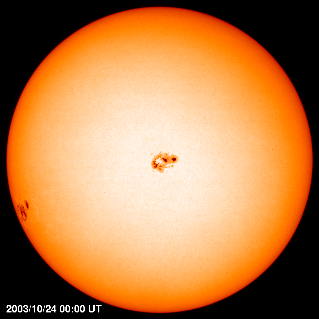
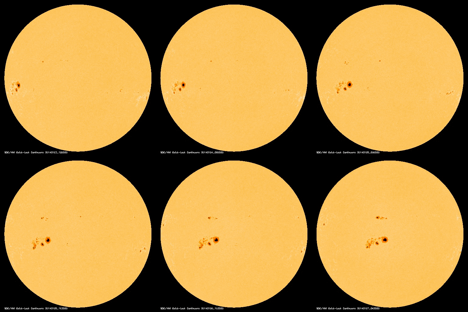
Now we have all the information needed except for the Sun's rotation around its own axis. Following Galileo's example, we can use sunspots as tracers of the Sun's rotation

Source

Unfortunately, whenever my lab group checked, there were no large, obvious sunspots to track. Instead, we used previously recorded video data (much like the gif above) to track sunspots over time. I tracked three sunspots from 2001:

The top sunspot traveled:

• 51 degrees in 3:12:48 days = 305280 seconds
• 53 degrees in 3:17:36 days = 322560 seconds
• The average is 52 degrees in \(3.14 \times 10^5\) seconds (pi!), giving a period of: \[ \frac{P}{360^{\circ}} =  \frac{seconds \: traveled }{degrees \: traveled} \] \[ P =  \frac{3.14 \times 10^5 \times 360^{\circ}}{52^{\circ}} = 2.17 \times 10^6 s\]

The middle sunspot traveled:

• 50 degrees in 3:12:48 days = 305280 seconds
• 40 degrees in 2:17:36 days = 236160 seconds
• The average is 45 degrees in \(2.71 \times 10^5 \) seconds, giving a period of: \[ \frac{P}{360^{\circ}} =  \frac{seconds \: traveled }{degrees \: traveled} \] \[ P =  \frac{2.71 \times 10^5 \times 360^{\circ}}{45^{\circ}} = 2.17 \times 10^6 s\]

The bottom sunspot traveled:

• 83 degrees in 6:19:12 days = 587520 seconds
• 30 degrees in 2:11:12 days = 213120 seconds
• The average is 56.5 degrees in \(4.00 \times 10^5 \) seconds, giving a period of: \[ \frac{P}{360^{\circ}} =  \frac{seconds \: traveled}{degrees \: traveled} \] \[ P =  \frac{4.00 \times 10^5 \times 360^{\circ}}{56.5^{\circ}} = 2.52 \times 10^6 s\]

The average is \(2.29 \times 10^6 s \) or 26.5 days. Interestingly, the first two spots were very consistent and decently close to the actual rotational period of the Sun (24.47 days) and the bottom sunspot was significantly farther than the other two data points. Alas, we cannot throw out data just because we know it is off and get a more accurate answer. However, we can pay attention to this discrepancy as a potential source of error.

Due to a lab group of uneven numbers, I worked on this section alone.