Exoplanet found with rings to put Saturn to shame.

I'm going to just start with the picture, because this planet is incredible:

Source

This is J1406b, a planet circling the star (you guessed it) J1406 and is the first exoplanet to be discovered with rings outside of our solar system. But this planet does not just have any rings; its ring system is about 200 times larger than Saturn's. The planet was described by the lead astronomer on the project, Eric Mamajek, as a "super Saturn." The massive ring system blocks about 95% of the light emitted by the sun-like star it is circling. This is how astronomers found the ring system, by studying the "eclipses" it produced with its star.

The ring system is expected to thin out over the next several million years as satellites form from the dust collecting. This planet can provide interesting insights to early versions of our solar system, before moons and satellites became more developed around our own planets.

Worksheet 7: All of it.

An Intro to Hydrostatic Equilibrium

The problem: Consider the Earth’s atmosphere by assuming the constituent particles comprise an ideal gas, such that P = nkT, where n is the number density of particles (with units cm^3 ), k = 1.4x10^16 erg K^1 is the Boltzmann constant. We’ll use this ideal gas law in just a bit, but first

Part A: Think of a small, cylindrical parcel of gas, with the axis running vertically in the Earth’s atmosphere. The parcel sits a distance r from the Earth’s center, and the parcel’s size is defined by a height ∆r + r and a circular cross-sectional area A (it’s okay to use r here, because it is an intrinsic property of the atmosphere). The parcel will feel pressure pushing up from gas below (Pup = P(r)) and down from above (Pdown = P(r + ∆r)).

Part B: What other force will the parcel feel, assuming it has a density ρ(r) and the Earth has a mass M?

The parcel will also feel gravitational force, which we will denote as \(\vec{F_g}\).

Part C: If the parcel is not moving, give a mathematical expression relating the various forces, remembering that force is a vector and pressure is a force per unit area.

If the parcel is not moving, we can conclude: \[\vec{F_{up}} + \vec{F_{down}} + \vec{F_g} = 0\] And because pressure is force per unit area, we have \[A\vec{P_{up}} +A \vec{P_{down}} + \vec{F_g} = 0\]

Part D: Give an expression for the gravitational acceleration, g, at at a distance r above the Earth’s center in terms of the physical variables of this situation.

We know that the equation for gravity is: \[F_g = - \frac{GM_{\oplus}M_{gas}}{r^2}\] Using F=ma or in this case, F=mg, allows us to solve for g. \[M_{gas}g= - \frac{GM_{\oplus}M_{gas}}{r^2}\] \[g(r)= - \frac{GM_{\oplus}}{r^2}\] 

Part E: Show that \[\frac{dP}{dr} = - \rho g \] is the equation of hydrostatic equilibrium.

We can rewrite F to give: \[F_g= V \rho g\] where \[V = \Delta r A\] so \[F_g=\Delta r A \rho g\] We can also rewrite the equation found in part C to give \[F_{up} + F_{down}= -F_g\] Plugging in pressures and our new form of F allows us to solve:\[AP(r) - AP( \Delta r + r ) = - \Delta r A \rho g \]\[P(r) - P( \Delta r + r ) = - \Delta r  \rho g \] \[P(r) - P( \Delta r + r ) = - \Delta r  \rho g \]  \[\frac{P(r) - P( \Delta r + r ) }{\Delta r} = - \rho g \] \[ \lim_{r\to\infty} \frac{P(r) - P( \Delta r + r ) }{\Delta r} = - \rho g \] \[\frac{dP}{dr} = - \rho g \] 

Part F: Now go back to the ideal gas law described above. Derive an expression describing how the density of the Earth’s atmosphere varies with height, ρ(r)? (HINT: It may be useful to recall that dx/x = d ln x.)

Because \[n = \frac{particles}{cm^3}\] \[\rho = \frac{ \bar{m} particles}{cm^2}\] \[ \rho = \bar{m} n\] \[n= \bar{m} \rho\] Therefore using P=nkT gives: \[P = kT \frac{\rho}{ \bar{m}}\] Plugging this back into \[\frac{dP}{dr} = - \rho g \] gives \[ \frac{d (kT \frac{ \rho}{ \bar{m} })}{dr} = - \rho g \] \[\frac{kT}{ \bar{m}} \frac{d ( \rho)}{\rho} = - g dr \] Which we can integrate to find the answer \[\frac{kT}{ \bar{m}} \int \frac{d ( \rho)}{\rho} = \int - g dr \]  \[\frac{kT}{ \bar{m}} ln(\rho) = - g r + C \] \[ \rho (r) = C \cdot e^{\frac{-gr \bar{m} }{kT}} \]

Part G: Show that the height, H, over which the density falls off by an factor of 1/e is given by \[H= \frac{kT}{g \bar{m}}\] where m is the mean (average) mass of a gas particle. This is the “scale height.” First, check the units. Then do the math. Then make sure it makes physical sense, e.g. what do you think should happen when you increase m? Finally, pat yourselves on the back for solving a first-order differential equation and finding a key physical result!

First check units: \[H_{units} = cm \] \[H_{units} = \frac{ \frac{gcm^2}{ks^2} \cdot k}{ g \cdot \frac{cm}{s^2}} = cm \]

Now we can solve. The problem is asking for us to solve for the scenario below:

In the equation found in F, when H=0 \[ \rho (r) = C \cdot e^{0}  = C\] so the equation can be written as \[ \rho (r) = \rho_{\circ}  \cdot e^{\frac{-gr \bar{m} }{kT}} \] For this problem we need \[ \frac{\rho (r) }{\rho_{\circ}} = e^{-1} \] So \[ -1 = \frac{-gH \bar{m}}{kT} \] Solving for H gives the answer \[H= \frac{kT}{g \bar{m}}\]

This makes physical sense because if the mean mass of a gas particle gets heavier, the scale height should be lower. 

Part H: What is the Earth’s scale height, \(H_{\oplus}\)? The mass of a proton is 1.7 x 10^-24 g, and the Earth’s atmosphere is mostly molecular nitrogen, N2, where atomic nitrogen has 7 protons, 7 neutrons.  

Assuming an outside temperature of 300 kelvin and that \(N_2\) has 28 photons and neutrons of the same mass  \[\bar{m} =  28 \times 1.7 \times 10^{-24} = 4.8 \times 10^{-23} \]  Then solve \[H_{\oplus}= \frac{kT}{g \bar{m}}\] \[H_{\oplus}= \frac{1.4 \times 10^{-16} \times 300}{1000 \times 4.8 \times 10^{-23} \times 14 } = 8.8 \times 10^5 cm \]

Acknowledgements: I worked with Barra on this problem.

Worksheet 6, Problem 2; Temperature of the Sun

The problem: Consider the amount of energy produced by the Sun per unit time, also known as the bolometric luminosity, \(L_\odot\). That same amount of energy per time is present at the surface of all spheres centered on the Sun at distances r > \(R_\odot\). However, the flux at a given patch on the surface of these spheres depends on r. (The Stefan-Boltzmann Constant: σ = 5.7 x \(10^5 erg cm^2 s^{-1} K^4 \))
(a) How does flux, F, depend on luminosity, L, and distance, r?
(b) The Solar flux at the Earth-Sun distance has been measured to high precision, and for the purposes of this exercise is given by \(F_\odot = 1.4 x 10^6 erg cm^2 s^{-1}\) . Given that the Sun’s angular diameter is θ = 0.57 degrees, what is the effective temperature of the Sun? (HINT: start with the mathematical version of the first sentence of this problem, namely,\[L_\odot (r = R_\odot) = L_\odot (r = 1 AU) \] and then expand the left and right sides in terms of their respective distances, r, and fluxes at those distances.)


What we know:

• \(F_\odot = 1.4 x 10^6 erg cm^2 s^{-1}\) 
• \(L_\odot = 4 \pi R_\odot^2  σ T^4\)
• \(F = σ T^4\)
• θ = 0.57 degrees, which we can use to calculate the actual diameter of the sun

\[tan(0.57) = \frac{x}{1.5 x 10^{13}} \: x = tan(0.57) \cdot 1.5 x 10^{13}\] for small angles we can approximate tan(θ) as θ in radians so tan(.57) in radians is: \[.57\,^{\circ} \cdot \frac{2 \pi}{360\,^{\circ}} = \frac{.57 \pi}{180}\] and the radius of the sun is: \[R_\odot \approx \frac{1.5 x 10^{13}}{2} \cdot \frac{57 \pi}{180} \approx 7.5 x 10^{10}cm\]

Solve:

Part A:

• We know the units of F is \(\frac{erg}{s\:cm^2}\) and L is \(\frac{erg}{s} \) and A is \(cm^2\)

We can therefore conclude that we can use the relationship \[F= \frac{L}{A_E} \] where A is the area where the sun is isotropically emitting energy with the radius being the distance from the sun to Earth so \[A_r = 4 \pi d_E^2\] which gives \[F = \frac{L}{ 4 \pi d_E^2}\]

Part B:
We know \(L_\odot = 4 \pi R_\odot^2  T_\odot^4 \sigma\) and solving for luminosity gives \[L_\odot= F_\odot 4 \pi d_E^2\] \[4 \pi R_\odot^2  T_\odot^4 \sigma =F \cdot 4 \pi d_E^2\] and we can solve for temperature: \[T_\odot^4 = \frac{F_\odot 4 \pi d_E^2}{ 4 \pi R_\odot^2  \sigma }\] \[T_\odot = \sqrt[4]{\frac{F_\odot d_E^2}{ R_\odot^2  \sigma }}\] Plugging in all out givens allows us to solve: \[T_\odot = \sqrt[4]{\frac{1.4 x 10^6  \cdot  (1.5 x 10^{13})^2}{ (7.5 x 10^{10})^2 (5.7 x 10^{-5} )}}\]\[T_\odot = 5.6 x 10^3 \:K \]

Acknowledgements: I worked with Barra and April on this problem.

Worksheet 5, Problem 2: Setting up important equations

The problem: Blackbodies are nice because they’re such simple objects. Their outward appearance is entirely determined by their temperature. If there were cows in space, astronomers would imagine them to be spherical blackbodies (and seriously, it wouldn’t be a bad approximation). In this exercise we’ll take advantage of the relative simplicity of blackbodies to derive some useful expressions that you’ll use during this term, and throughout your astronomy career.

Part A: In astronomy, it is often useful to deal with something called the “bolometric flux,” or the energy per area per time, independent of frequency. Integrate the blackbody flux Fν(T) over all frequencies to obtain the bolometric flux emitted from a blackbody, F(T). You can do this using by substituting the variable u = hν/kT. This will allow you to split things into a temperature-dependent term, and a term comprising an integral over all frequencies. However, rather than solving for the integral, just set the integral and all constants equal to a new, single constant called σ, which is also known as the Stefan-Boltzmann constant. If you’re really into calculus, go ahead and show that \(σ \approx 5.7 x 10^5 erg s^{-1} cm^{-2} K^{-4}\) . Otherwise, commit this number to memory.

In question 1 on this worksheet we found that \[F_ν(T) = \frac{2 \pi ν^3h}{c^2 (e^{ \frac{hv}{kT}} - 1 )}\] for this problem we need \[F(T) = \int_{0}^{\infty} \frac{2 \pi ν^3h}{c^2 (e^{ \frac{hv}{kT}} - 1 )}\] where \[ u = \frac{hν}{kT} \: and\: dν = \frac{h}{kT} dν\] so substituting u in for every instance of ν gives \[F(T) = \frac{2 \pi K^4}{c^2h^3} \cdot \int_{0}^{\infty} \frac{T^4 u^3}{e^u - 1} du\] as per the problem's instructions, we can set sigma equal to the integral and all constants:  \[σ  = \frac{2 \pi K^4}{c^2h^3} \cdot \int_{0}^{\infty} \frac{u^3}{e^u - 1} du\] therefore \[F(T) = σ T^4\]

Part B: The Wien Displacement Law: Convert the units of the blackbody intensity from Bν(T) to Bλ(T) IMPORTANT: Remember that the amount of energy in a frequency interval dν has to be exactly equal to the amount of energy in the corresponding wavelength interval dλ.

Mathematically, the problem is telling us that \[B_ν \cdot dν = B_λ \cdot dλ\] or \[B_λ = B_ν \frac{dν}{dλ}\] We also know from previous problems that \[ ν = \frac{c}{λ}\] which gives: \[\frac{dν}{dλ} = -  \frac{c}{λ^2}\] Plugging these values into the above equation gives: \[B_λ = -\frac{2 \left( \frac{c}{λ} \right)^3}{c^2} \cdot  \frac{h \left( \frac{c}{λ} \right)}{e^{\left( \frac{hc}{kTλ} \right)} -1} \cdot \frac{c}{λ^2} \] which simplifies to \[B_λ(T) = \frac{-2hc^2}{λ^5 \left( e^{\left( \frac{hc}{kTλ} \right)} -1 \right)} \]

Part C: Derive an expression for the wavelength λmax corresponding to the peak of the intensity distribution at a given temperature T. (HINT: How do you find the maximum of a function?) Once you do this, again substitute \(u = \frac{hν}{kT}\). The expression you end up with will be transentental, but you can solve it easily to first order, which is good enough for this exercise.

Beware: There are a lot of equations ahead.

So basically we can take the derivative of the below equation to find the maximum wavelength. \[B_λ(T) = \frac{-2hc^2}{λ^5 \left( e^{\left( \frac{hc}{kTλ} \right)} -1 \right)} \] using \[ u = \frac{hc}{kTλ} and λ = \frac{kT}{hcu} \] which gives us: \[B_λ(T) = \frac{-2K^5T^5u^5}{h^4c^3(e^u - 1)} \] taking the derivative gives: \[B_λ(T) = \frac{h^4c^3(e^u-1)(-10K^5u^4) + (2K^5T^5u^4) + 2k^5T^5u^5(h^4e^3e^u)}{(h^4c^3e^u - h^4c^3)^2} \] which when set equal to zero amazingly enough simplifies to \[e^u(u-5) = -5\]. Because it is difficult to solve, we can approximate u with a taylor expansion \( e^x \approx 1 + x \). \[(1-u)(u-5) = -5\]\[u=4\] Plugging back into the original equation for λ gives the maximum wavelength: \[λ_{max}= \frac {hc}{4kT} \]

Part D: The Rayleigh-Jeans Tail: Next, let’s consider photon energies that are much smaller than the thermal energy. Use a first-order Taylor expansion on the term \(e^{\frac{hν}{kT}}\) to derive a simplified form of Bν(T) in this low-energy regime. (HINT: The Taylor expansion of \( e^x \approx 1 + x \) ).
If \[e^x \approx 1 + x \] then \[e^{\left( \frac{hν}{kT} \right)} \approx 1 +\frac{hν}{kT} \] plugging this into the given equation gives: \[B_ν(T) = \frac{2ν^2}{c^2} \frac{hv}{1 + \frac{hν}{kT} -1} \] which simplifies to:  \[B_ν(T) = \frac{2ν^2kT}{c^2}\].

Part E: Write an expression for the total power output of a blackbody with a radius R, starting with the expression for Fν. This total energy output per unit time is also known as the bolometric luminosity, L.

We know the units of F is \(\frac{erg}{s\:cm^2}\) and L is \(\frac{erg}{s} \) and A is \(cm^2\)

We can therefore conclude that we can use the relationship \[F= \frac{L}{A} \] where A is the area where the blackbody is isotropically emitting energy with the radius, R, being the distance away from the blackbody so \[A_r = 4 \pi R^2\] which gives \[L= \frac{F}{ 4 \pi R^2}\] and \[ L = σ T^4 4 \pi R^2\]

Acknowledgements: A huge thank you to Barra for doing this problem with me and to John for guiding us in TALC.

The Mystery of the Disappearing Star

Last month, Popular Science released an article  based on a paper in The Astrophysical Journal about a star that astronomer have been studying for the past years that has recently seemingly disappeared. So how does one misplace a star?

The star is actually a pulsar, or a "rotating neutron star, the result of a massive star collapsing in on itself." It emits beams of electromagnetic radiation that astronomers can observe and use to track the pulsar.

Source

The star also makes up half of a binary star system called J1906, rotating around another star, which leads to how the star "disappeared." The mass of the companion star creates a "sinkhole" in space-time. Now the pulsar's radio waves cannot reach Earth and the star has become unobservable. 

Source

This phenomena is called geodetic precession. Einstein's theory of relativity can explain how the star's axis is tilted by the warp in space-time, until the previously visible radiation is no longer visible on Earth. 

Fear not, the pulsar is estimated to be visible again in less than 160 years.

Worksheet 4, Problem 2: The bigger, the better?

The problem: CCAT is a 25-meter telescope that will detect light with wavelengths up to 850 microns. How does the angular resolution of this huge telescope compare to the angular resolution of the much smaller MMT 6.5-meter telescope observing in the infrared J-band? Ask a TF in class or the internet about the meaning of “J-band.”

What we know:

• From class, we know the equation of angular resolution is: \[\theta_{min} \approx \frac{\lambda}{D}\] where the lambda is the wavelength of light and D is the diameter of a telescope mirror.

Source

• From the internet we know "In infrared astronomy, the J band refers to an atmospheric transmission window centred on 1.25 micrometres(in the near-infrared)." (Source) 
• A micron is the same thing as a micrometer, both equivalent to \( 1 x 10^{-4} cm\).

Solve:

For CCAT: \[\theta_{CCAT} \approx \frac{8.5 x 10^{-2} cm }{2.5  x 10^{3} cm} \approx 3.4  x 10^{-5} radians \]
For MMT:\[\theta_{MMT} \approx \frac{1.25 x 10^{-4} cm }{6.5  x 10^{2} cm} \approx 1.9 x 10^{-7}radians \]

Update:

Converting these answers to arcseconds gives:
\[\theta_{CCAT}  \approx 3.4  x 10^{-5} radians \cdot \frac{2 \times 10^5 \: arcsecond}{1 \: radian} \approx  6.8 \: arcseconds\]

\[\theta_{MMT} \approx 1.9 x 10^{-7} radians  \cdot \frac{2 \times 10^5 \: arcsecond}{1 \: radian} \approx  3.8 \times 10^{-2} \: arcseconds\]

This exemplifies the relationship in the equation: when diameter is bigger, the angular resolution is smaller. In this case, the MMT angular resolution is about 100 times smaller than the angular resolution for CCAT.
]'[

Acknowledgements: Thanks to Barra, Eden, and April for struggling through this worksheet with me and to Andrew for helping us at TALC.

Bonus: Here is a CCAT telescope (Source) and an MMT telescope (Source).

Worksheet 4, Problem 1: Telescopes are much more complex than they appear

The problem: To understand the basics of astronomical instrumentation, I find it useful to go back to the classic Young’s double slit experiment. Draw a double slit setup as a 1-D diagram on the board. Draw it big, use straight lines, and label features clearly. The two slits are separated by a distance D, and each slit is w wide, where w << D such that its transmission function is basically a delta function. There is a phosphorescent screen placed a distance L away from the slits, where L >> D. We’ll be thinking of light as plane-parallel waves incident on the slit-plane, with a propagation direction perpendicular to the slit plane. Further, the light is monochromatic with a wavelength λ.
a) Convince yourself that the brightness pattern of light on the screen is a cosine function. (HINT: Think about the conditions for constructive and destructive interference of the light waves emerging from each slit).
b) Now imagine a second set of slits placed just inward of the first set. How does the second set of slits modify the brightness pattern on the screen?
c) Imagine a continuous set of slit pairs with ever decreasing separation. What is the resulting brightness pattern?
d) Notice that this continuous set of slits forms a “top hat” transmission function. What is the Fourier transform of a top hat, and how does this compare to your sum from the previous step?
e) For the top hat function’s FT, what is the relationship between the distance between the first nulls and the width of the top hat (HINT: it involves the wavelength of light and the width of the aperture)? Express your result as a proportionality in terms of only the wavelength of light λ and the diameter of the top hat D.
f) Take a step back and think about what I’m trying to teach you with this activity, and how it relates to a telescope primary mirror.

Simple, right? Let's take this one step at a time.

What we know:

Source

Young's double slit experiment is set up as shown above, with light going through a screen with two slits, interacting and creating a subsequent pattern on the screen a distance, L, away. We will find out more about what happens as we go through the problem.

Part A: Convince yourself that the brightness pattern of light on the screen is a cosine function. (HINT: Think about the conditions for constructive and destructive interference of the light waves emerging from each slit).

First we must think about the nature of waves. When two waves interact with each other they overlap, creating constructive interference (where both waves add to each other) and destructive interference (where the two waves cancel each other out) as shown below.

Source

So visually, we can see the cosine pattern, up and down. If this does not seem like a sufficient explanation, we can turn to a mathematical explanation. In this week's reading (or viewing) we learned how the resultant interactions of two waves of light cause destructive and constructive interference in a sine (or cosine) function shown by the trigonometry written out below:

Source

Where if n is a whole integer there is constructive interference as the wavelengths add together and destructive interference in between where half-wavelengths for r cancel each other out.

Part B: Now imagine a second set of slits placed just inward of the first set. How does the second set of slits modify the brightness pattern on the screen? 

So we set up the experiment as shown below, but how do we get to the shown pattern?

Source

Well, we know the first set of slits gives a cosine pattern. The second, inner set of slits would also give a cosine pattern, yet with a larger period. This is supported by the given equation \[ y \propto

 n \cdot L \cdot \frac{\lambda}{D}\] where y is the distance between maxima, so with a smaller distance between slits, the distance between maxima is greater.

Now all we have to do is add the two cosine functions:

and we get a new brightness pattern for four slits as shown above, with more intense spots of constructive interference.

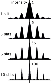
Part C: Imagine a continuous set of slit pairs with ever decreasing separation. What is the resulting brightness pattern?

This means adding more and more cosine functions

until you get:

Source

Eventually, adding all these slit pairs will give one, large slit with increasing intensity in the center that looks something like the image below:

Source

Part D: Notice that this continuous set of slits forms a “top hat” transmission function. What is the Fourier transform of a top hat, and how does this compare to your sum from the previous step?

The Fourier transform gives us a Sinc pattern of brightness, which looks like our sum from the previous step.

Source

Part E: For the top hat function’s FT, what is the relationship between the distance between the first nulls and the width of the top hat (HINT: it involves the wavelength of light and the width of the aperture)? Express your result as a proportionality in terms of only the wavelength of light λ and the diameter of the top hat D.

To understand this question, we have to know what W represents in the image above. W is a dimensionless quantity that describes how many wavelengths wide a gap, D, is. We can define this as: \[W = \frac{D}{\lambda} \]

To find the distance between two nulls, we can use the image above and see that it would be twice of \(\frac{1}{W}\) giving us: \[distance = \frac{2}{W} \: or \: distance = \frac{2\lambda}{D}\]

Part F: Take a step back and think about what I’m trying to teach you with this activity, and how it relates to a telescope primary mirror.

We can think of the mirror on a telescope as a single slit diffraction experiment:

Source

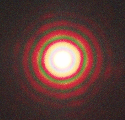
In reality, the light would bounce back from the mirror, but it is easier to represent it "passing through" like a single slit. The "slit" (really the mirror) blocks out all light on the sides, takes in some light and allows it to spread, amplify, and gain intensity. Essentially, we can then see something as "bigger" than with our naked eye. Due to the previously discussed interference patterns, powerful telescope would show a star not as a point of light, but as an interference pattern like below:

Source

Acknowledgements: Thanks to Barra and Eden for struggling through this worksheet with me and to Andrew for helping us at TALC.

If light travels so fast, why does this video feel so slow?

For my first free-form blog post, I wanted to share a video I saw last week that blew my mind, just very slowly.

The video shows the reality of what it would be like to traverse our solar system at the speed of light. Cool, right? We get to travel as fast as the fastest known wave-particle in our universe. Sit back and enjoy the ride. I expected the video to go something like this gif below:

Source: http://www.huffingtonpost.com/2015/02/02/riding-light-video_n_6595092.html

And yet the video (which can be found at the link above) is 45 minutes long, and that's not even our entire solar system. Only at 43 minutes do we reach Jupiter, and if you want to see Saturn, you'll have to sit through another 35 minutes of video.

So, why do we care?

Conceptually, I knew that it takes light 8 minutes to get to the Earth, but that is just a fact I memorized at some point in middle school. There is nothing like sitting through 8 minutes of video to really hone that fact in (though I honestly watched 30 seconds and skipped ahead). Yet the speed of light is so large.  \[3 \cdot 10^{10} \frac{cm}{sec}\]

Which must mean our solar system is big, really big. Once again, this is something we all know, but I'm not sure can truly appreciate. Growing up with models like the one below:

Source: https://www.ou.org/jewish_action/02/2013/the-big-pang-theory/solar-system/

Are great for teaching elementary school kids about the planets, but leave us with a wildly inaccurate model of space. No matter how many facts we memorize or distances we compute, there is nothing like seeing it yourself to subvert the inaccurate models we grew up with. Today in class, Professor Johnson said that no one is born with an instinct for astronomy, and I think this article goes to show how important our methods of learning are for understanding our universe.

Acknowledgements: Although I have included the link twice already, for good measure, the video and article I discuss can be found at http://www.huffingtonpost.com/2015/02/02/riding-light-video_n_6595092.html.

Worksheet 3, Problem 3: Stargazing Monthly

The problem: Consider the star AY Sixteenus, located at RA = 18 hours and Dec = +32 degrees. On the first of each month, at what LST is AY Sixteenus on the meridian as viewed from Cambridge, MA (latitude 42 degrees, longitude of 71 degrees West)? On what date is the star on the meridian at midnight LST?

What we know: Right ascension (RA) and declination (Dec) are a coordinate system for celestial objects that correspond with longitude and latitude respectively. Because the problem only concerns the location of AY Sixteenus relative to our Meridian, we can ignore declination for the sake of this problem. Consequently, let's look closer at RA:

Image from: http://en.wikipedia.org/wiki/Right_ascension

Right ascension is measured eastward from the vernal equinox, which we know from question 2, has the unique property of being 00:00 LST at noon on March 20th.

Solve: With the background information we know, the first part of the problem seems much easier, almost a trick. If the RA of the star is 18, its LST will always be 18:00 hours, regardless of the day of the year. So the star will be at 18:00 LST on the first of every month. The thing that does change, however is at what time the star is on our meridian.

So now we can tackle the last part of the problem. We need to find when the star would be on our meridian at midnight solar time (this is my interpretation, confirmed by John during TALC). To visualize this we can draw another diagram.

Because the star is 18 hours away from 0, if we convert that to degrees: \[18\: hours \cdot \frac{15\,^{\circ}}{1\:hour} = 270\,^{\circ}\] so that means that at 0:00 LST, the star is on the meridian of \(90\,^{\circ}\) W. Our longitude is only \(19\,^{\circ}\) away (because the Earth spins East) so the star will be on our meridian \[19,^{\circ} \cdot \frac{1\:hour}{15\,^{\circ}} \approx 1 \: hour \: 6\: min\] one hour and six minutes later at 19:06 LST, or 18 hr + 1 hr & 6 min from noon on March 20th. 19:06 sidereal hours from noon would be 7:09 UT (accepting a difference of 4 min a day).

Finally, all we need is to find is when the star would be on the meridian at midnight, local time. 7:09 UT would be 2:09 EST due to the five hour time difference. 2:09 in the morning is 9 hours 51 minutes from midnight or 591 minutes away from midnight (9 x 60 = 540 min + 51 min = 591 min). From problem 2, we can do the same 4 min/day conversion to find:\[591 \:min \cdot \frac{1 \: day}{4\:min} \approx 148\: days\] 148 days after March 21 would be August 16th!

Acknowledgements: Thanks to John for his help at TALC to get started on this problem.

Update: After another visit to TALC and another talk with John, I realized where I went wrong. I understood that LST was measured from Greenwich, like UTC, but that is incorrect because it is local standard time, measured from your location. Then we only have to correct for 6 hours, and at a rate of 2 hours a month, the star would be on our meridian 3 months after the vernal equinox. This would be around June 20th, not August 20th like I originally found.

Worksheet 3, Problem 1: A Day in the Life of a Martian

The problem: What is the difference between sidereal and solar day on Mars if Mars has the same rotation period and orbits at 1.5 AU.

What we know: We know a solar day on Mars is how long it takes for the sun to make a complete "rotation" in the sky and return to the same point. Because the Sun is not a fixed point in the sky (due to the fact that Earth and Mars are rotating it) a solar day will differ from a sidereal day, which is how long it takes for a fixed point (typically a star) to reach its same location in the sky.

Image from: http://ottawa-rasc.ca/articles/earl_mike/Satellite_Tracking/Dishes/Satellite_Dishes.html

We also know from Kepler's Law: \[P^2 \: \alpha \:  a^3 \]
and from the problem: \[P_e= 1 \: year\] \[a_e= 1\: AU\] \[a_m= \frac{3}{2} \: AU\](where \(P_e\) and \(P_m\) is the rotation period of the Earth and Mars respectively and \(a_e\) and \(a_m\) are the distance between the Sun and Earth and Mars respectively).

Solve:
From Kepler's Law we can set up the ratio: \[\frac{P_e^2}{P_m^2} = \frac{a_e^3}{a_m^3}\] and isolate the rotation period of Mars: \[P_m =\sqrt{\frac{P_e^2a_m^3}{a_e^3}}\] plugging in the provided values give:\[P_m =\sqrt{\frac{1^2\cdot \frac{3}{2}^3}{1^3}}\] which simplifies to: \[P_m=\left( \frac{3}{2} \right)^{\frac{3}{2}} \approx \frac{9}{5}\: Earth \:years\] when converting to days we get \[\frac{9}{5}\: Earth \:years \cdot 365 \: days \approx 660 \: days\: in \:a \:Martian\: year\] But this is not enough, we want the difference between the two days in minutes per day, not the length of a Martian year. To find the difference we can use the fact that Mars traverses an entire orbit in a 660 days \[\frac{360\,^{\circ}}{660 \:days} \approx \frac{0.55\,^{\circ}}{day}\] to show that a sidereal day is about half a degree less than a solar day. Then we can convert to days per minute: \[\frac{360\,^{\circ}}{660 \:days}\cdot \frac{1 \:hr}{15\,^{\circ}} \cdot \frac{60 \: min}{1 \: hr} \approx 2 \frac{min}{day}\]

Conclusion: with the given values, the difference between sidereal and solar day is about 2 minutes. This means that Mars's sidereal day is 2 minutes shorter than its solar day.

Acknowledgements: Many thanks to Barra for working on this worksheet with me.

Worksheet 2.1, Problem 4: Kepler's Law on a Desert Island

The problem: Using dimensional analysis alone, what is the form of Kepler’s law, which relates the period, total mass and separation of a two-body gravitational orbit? Use only the units and a tad of physics, e.g. what constants are likely involved?

What we have:

\[ P \: \alpha \: M\cdot a \] where P is period, M is mass, and a is the separation of a two-body gravitational orbit.

What we know:

Because gravity is involved, we know G will be used, which is \( G = 6.67 x 10^{-12}\frac{cm^3}{gs^2}\).

We also know the units:

Period: T (time), M: M (mass), a: L (distance) and finally G: \(\frac{L^3}{MT^2}\) (a combination of the three).

So we can set up a dimensional analysis problem with only the exponents to work out:

\[ P^w=M^x\cdot a^y\cdot G^z       \rightarrow      T^w=M^x\cdot L^y\cdot (\frac{L^3}{MT^2})^z\]

For the units of time (T) to balance out on both sides of the equation, w must equal 2 and z must equal -1. With this inversion, for the units for distance to work out (L), y must equal 3. And finally, for mass to cancel (M), x must equal -1.

In conclusion, w=2, x=-1, y=3, and z=-1, which when put back into the first equation gives:
\[ P^2=M^{-1}\cdot a^3\cdot G^{-1} \]

which cleans up to:
\[ P^2=\frac{a^3}{M\cdot G} \]

All done!

P.S. Because I do not live on a desert island, I looked up the formula for Kepler's law:
\[ P^2=\frac{4\pi^2 a^3}{MG} \]
and I was only off by a constant!

Many thanks to Sean and Eden for working on this worksheet with me.

Worksheet 2, Problem 2: The Power of a Distant Star

The problem: The eye must receive ~ 10 photons in order to send a signal to the brain that says, “Yep, I see that.” If you are standing in an enormous, completely dark cave and just barely discern a light bulb at a distance of 1 kilometer, what is the power output of the bulb?
Note: Assume the bulb is emitting light isotropically.
Note: The energy of a photon is E = hν, for a frequency ν (Greek letter ‘nu’), and Planck’s constant \(h = 6.6 x 10^{-27}\) erg/s.

Well, the problem is really:
What is the power output of a star that is 100 light years away that you can barely see from a dark site at night? Assume the star emits most of its energy at the peak of the eye’s sensitivity.

The only change here is that we have a more difficult conversion to get the distance between the star and our eye.

What we know:

• We know the speed of light is \(3 \cdot 10^{10} \frac{cm}{sec}\)
• We know there are \( 3.16 \cdot 10^7 \frac{sec}{year}\) from worksheet 2.2. \[ L = 100 \: years \cdot \frac{3.16 \cdot 10^7 \: sec}{year} \cdot  \frac{3 \cdot 10^{10} \:cm}{sec} \approx 9.5 \cdot 10^{19} \: cm \]
• E = hν
• \(P = \frac{\delta E}{\delta t}\)
• Visible light falls into a range between 390 - 700 nm, which an average could be 6.0 x \(10^{-7}\) cm.
• The radius of an eye is about 1 cm.
• The "refresh rate" of a movie is 50 Hz.

Solve:

Based on the fact that the light is emitted isotropically (shown partially in the diagram above), we can set up a ratio between the power emitted by the star over the area the light reaches to the power received by your eye to the area of your eye.\[\frac{P_{star}}{a_{light}} = \frac{P_{eye}}{a_{eye}}\]plugging in area formulas gives:\[\frac{P_{star}}{4 \pi L^2} = \frac{P_{eye}}{\pi r_{eye}^2}\] the main formula is now:\[P_{star} = \frac{P_{eye}\cdot 4 \pi L^2}{\pi r_{eye}^2 }\]

Now we all we need to find is the power reaching our eye, starting with finding the energy.  \[E = hv \: or \: E = h\frac{c}{\lambda} = 6.6 x 10^{-27} \cdot \frac{3 x 10^{10}}{6.0 x 10^{-7}} \approx 3.3x10^{-10} ergs\]

Now we need to find time. Something new I learned this week is refresh rate, or the rate at which movies emit light so that the brain does not notice any flickering in the movie. If the refresh rate of a movie is 50 Hz (\( \frac{1}{s}\)) and 10 photons must hit the eye every \( \frac{1}{50}\)s, so we need 500 photons a second. So the power would be  \[ P = \frac{500 photons}{sec} \cdot 3.3x10^{-10} ergs \approx 1.65x10^{-7} \frac{erg}{s}\] Plugging this into the original equation we get:\[P_{star} = \frac{1.65x10^{-7}\cdot 4 \pi (9.5 \cdot 10^{19})^2 }{\pi 1^2} \approx 5.9 \cdot 10^{33} \frac{erg}{s}\]

Update: The power output of a star is really just its luminosity \[L_{star} \approx 5.9 \cdot 10^{33} \frac{erg}{s}\] To check if our answer is reasonable we can compare that to the known luminsity of the sun \[L_{\odot} = 3.8 \times 10^{33} \frac{erg}{s} \] Because the luminosities are in the same order of magnitude, our answer seems reasonable.

Acknowledgements: Thanks to Sean and Eden for working on this problem with me and thanks to Fiona for explaining refresh rate to me.

Intro Post

Hi!!!

My name is Danielle Frostig (or Dani, or Frosting, or Frosted Flakes - I've heard them all and will respond to most). I am a freshman in Weld Hall from Southern California and still infinitely excited by all the snow. If you need to find me, I'll be outside making a snow angel.

I grew up on a college campus that has an observatory and once a month I got to go to the public visitor nights and use the big telescope, so my interest in astronomy was almost inevitable. This was further solidified by summer camps and research jobs, however my interest in astronomy wasn't always my only clear path. Before Harvard, I went to an arts school for six years studying visual arts like drawing, painting, and ceramics. I still absolutely love art, but ultimately decided to go to Harvard as an astrophysics major.

My love for astronomy only improved last semester after taking Astro 2- Celestial Navigation (so if school doesn't work out, I may become a pirate with my skills from that class) and after taking classes to get swipe access to the telescope. All this has made me more excited to take Astro 16.

I'll leave you with a picture of my high school graduation cap, which I think summarizes my interests pretty well.

Here's to a great semester!

Danielle